Why use activation functions?

Now that we understand what activation functions represent, and how some of them look, let’s discuss why we use activation functions in the first place. For a neural network to fit a nonlinear function, we need to have two or more hidden layers in the neural network, and we need those hidden layers to use a nonlinear activation function.

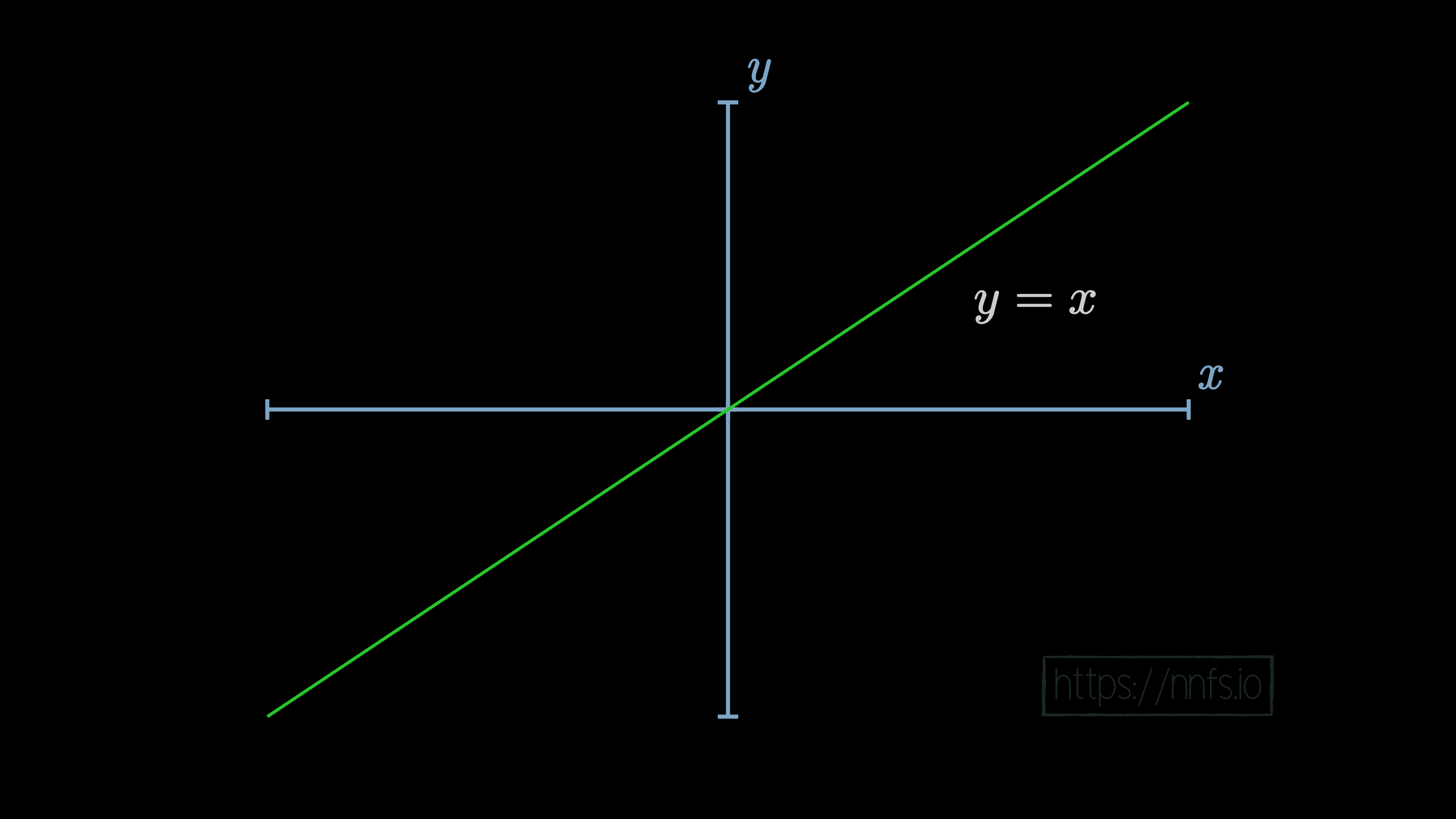
First off, what’s a linear and nonlinear function? A linear function is something like the equation of a line. If you graph it, it will present as a straight line on a graph. For example:

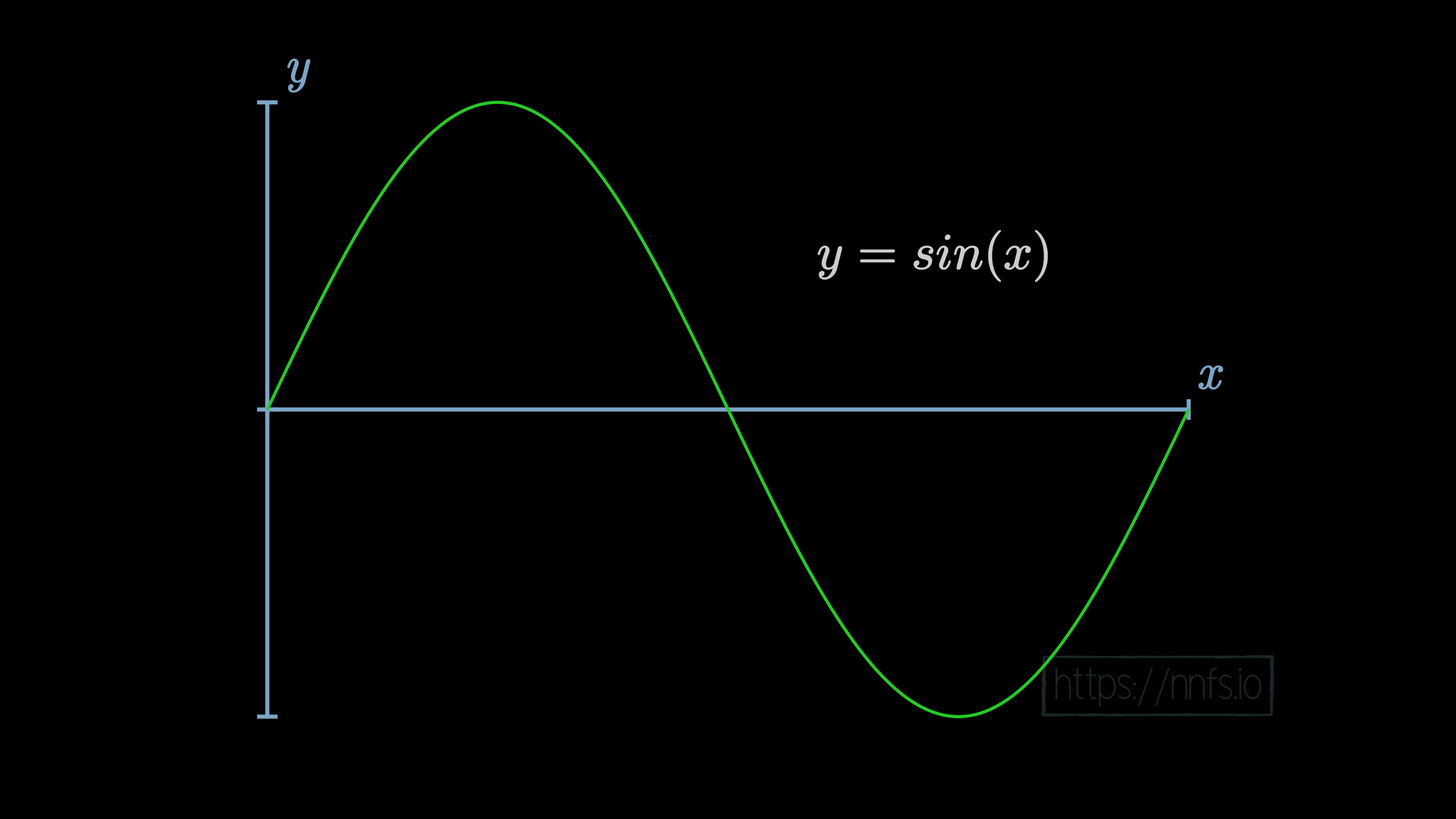
A nonlinear function cannot be represented well by a straight line, such as a sine function:

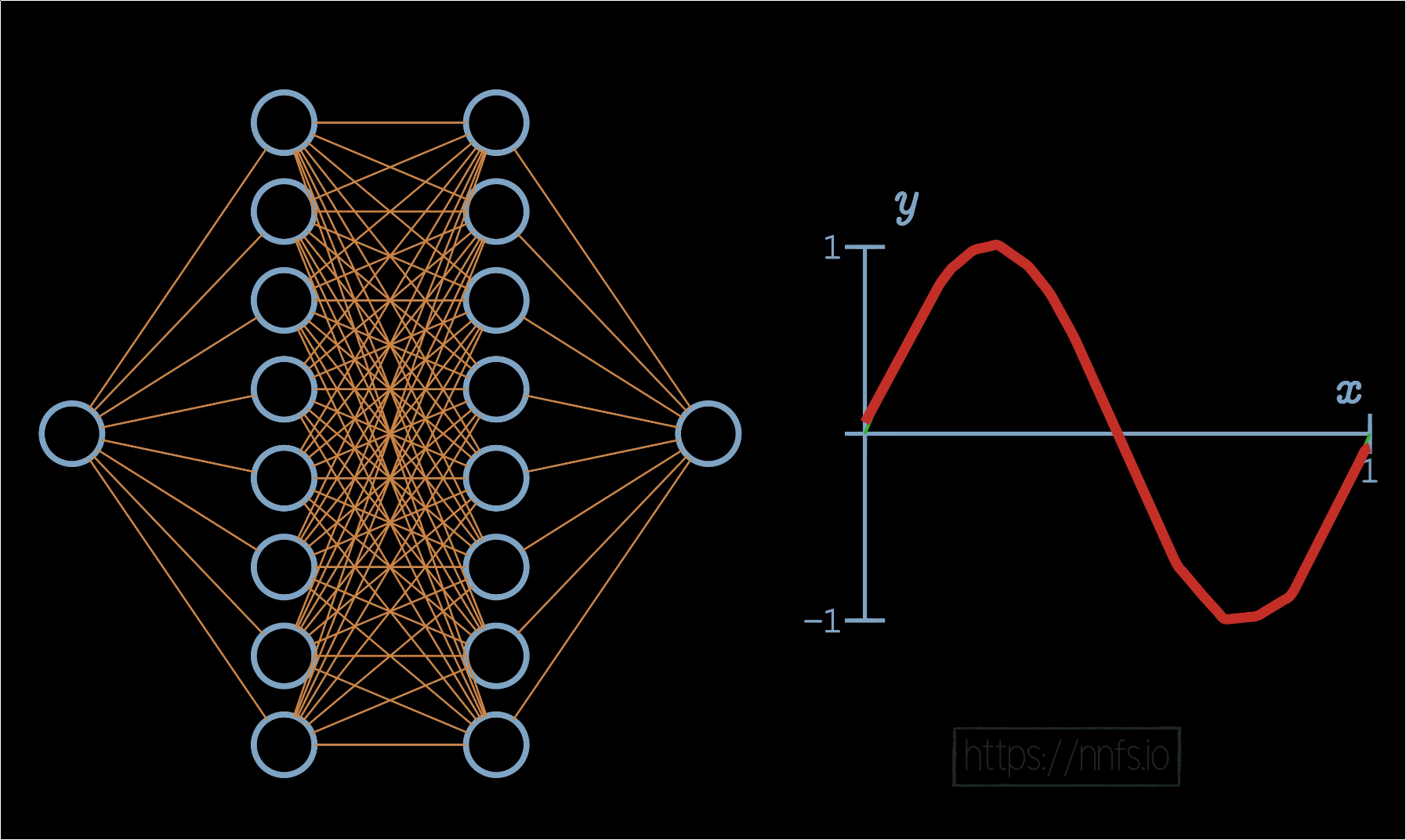
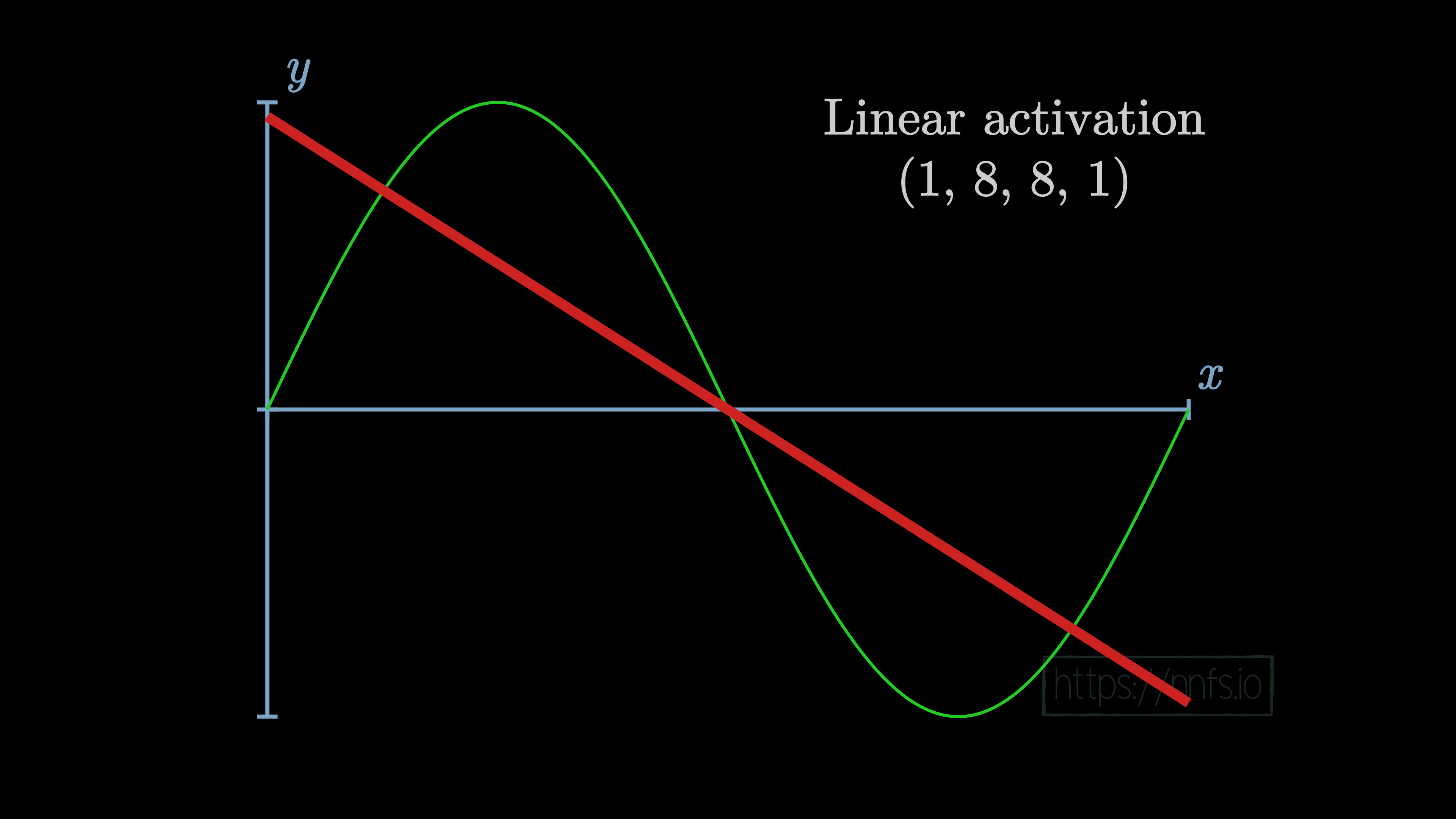
While there are certainly problems in life that are linear in nature, for example, if you’re trying to figure out the cost of some number of shirts, and we know the cost of an individual shirt, and that there are no bulk discounts, then the equation to calculate the price of any number of those products is a linear equation. Other problems in life are not so simple, like the price of a home. The number of factors that come into play, such as size, location, time of year attempting to sell, number of rooms, yard, neighborhood, and so on makes the pricing of a home a nonlinear equation. Many of the more interesting and hard problems of our time are nonlinear in nature. The main attraction for neural networks has to do with their ability to solve nonlinear problems. So first, let’s consider a situation where neurons have no activation function, which would be the same as having an activation function of y=x. With this linear activation function in a neural network with 2 hidden layers of 8 neurons each, the result of training this model will look like:

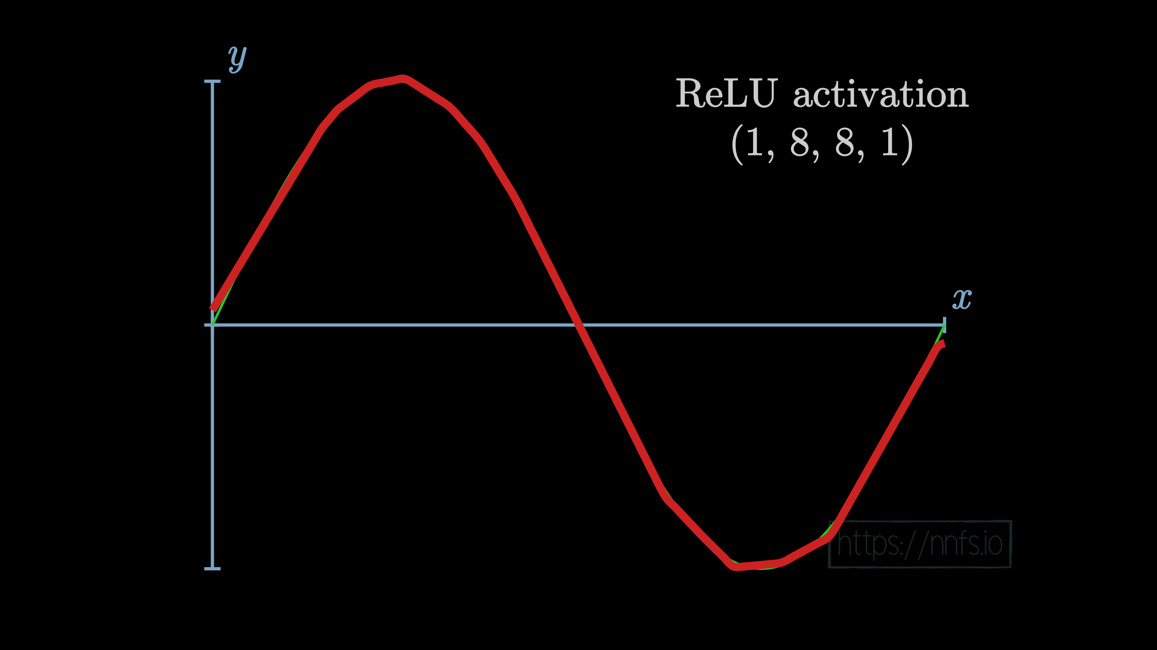
In the case of using the same 2 hidden layers of 8 neurons each, just with the rectified linear activation function, we see the following result after training:

Now that you can see that this is the case, we still should consider why this is the case. To begin, let’s revisit the linear activation function of y=x, and let’s consider this on a singular neuron level. Given values for weights and biases, what will the output be for a neuron with a y=x activation function? Let’s look at some examples:

As we continue to tweak with weights:

Weights and biases:

No matter what we do with this neuron’s weights and biases, the output of this neuron will be perfectly linear to y=x. This linear nature will continue throughout the entire network:

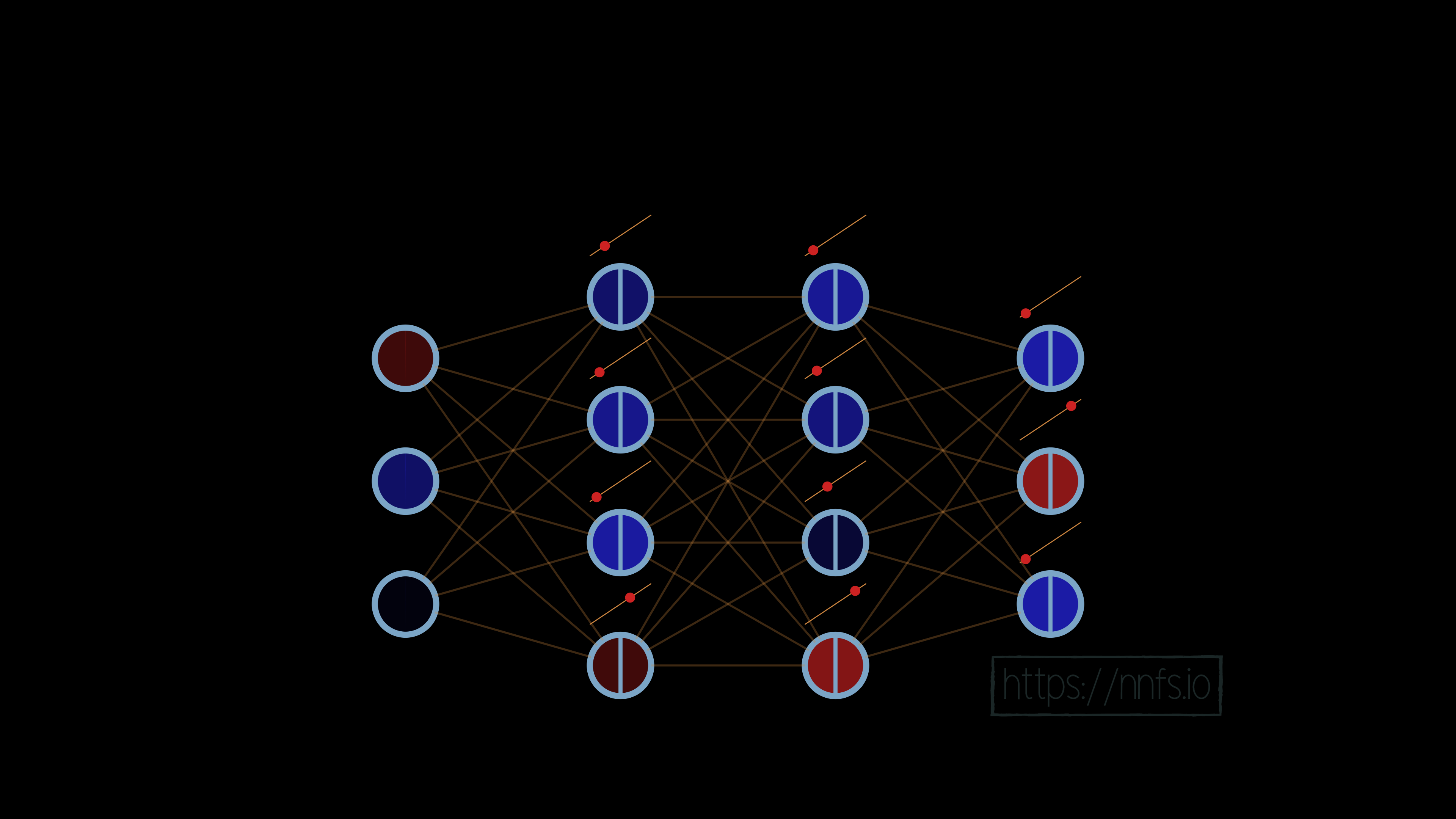
No matter what we do, however many layers we have, this network can only depict linear relationships if we use linear activation functions. It should be fairly obvious that this will be the case. We believe it is less obvious how, with a barely nonlinear activation function, like the rectified linear activation function, we can suddenly map nonlinear relationships and functions, so now let’s cover that. Let’s start again with a single neuron. We’ll begin with both a weight of 0 and a bias of 0:

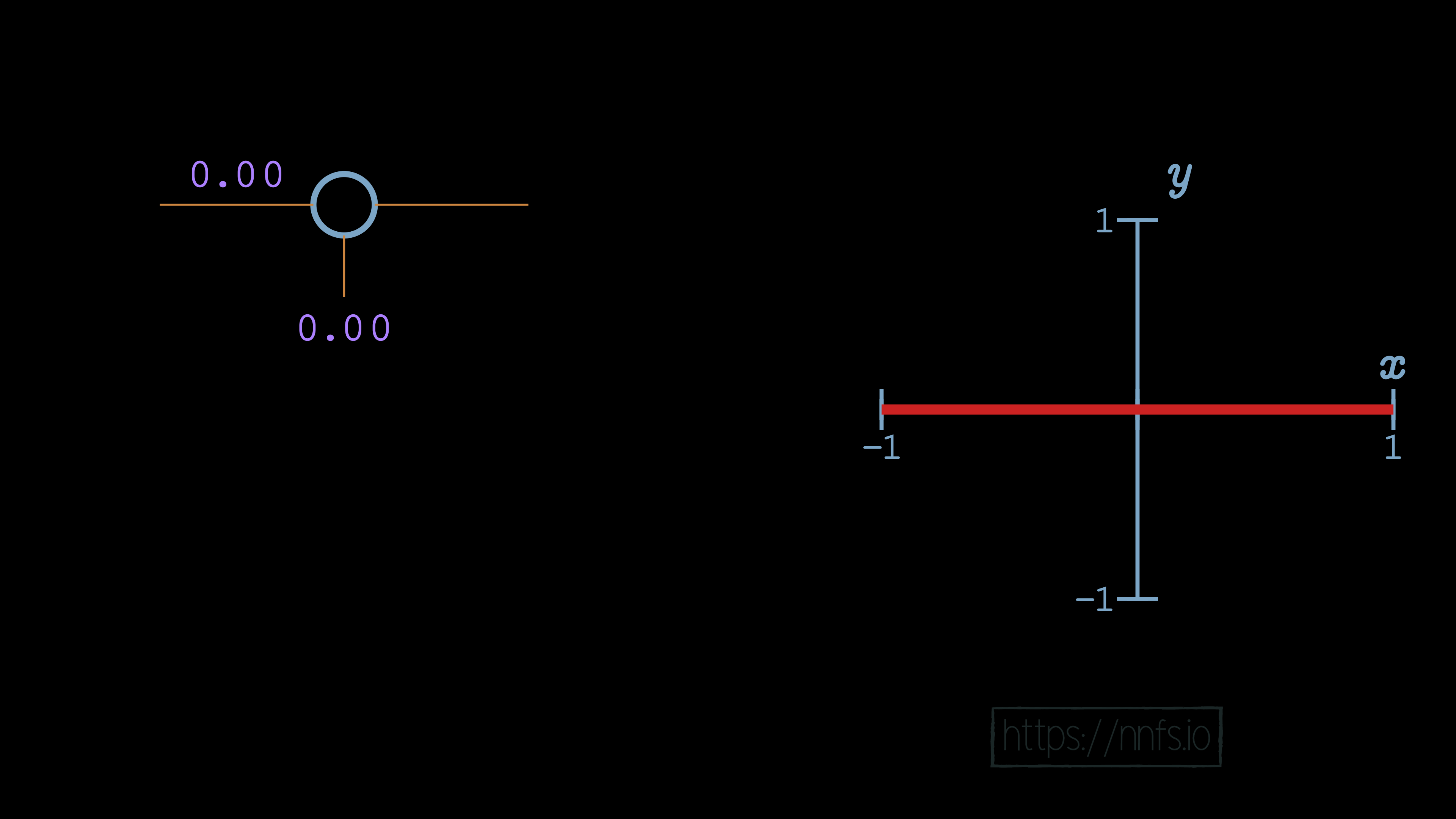
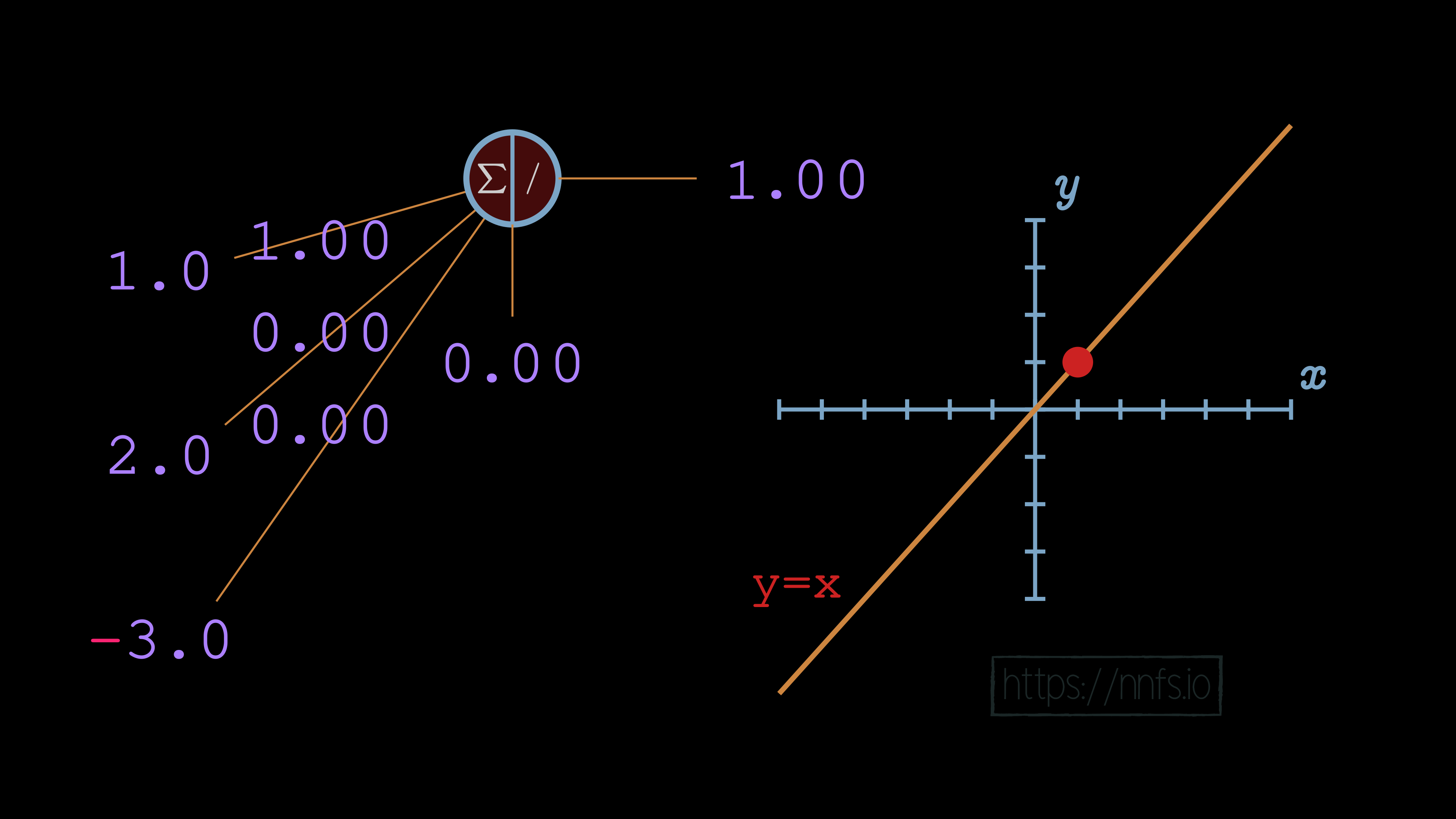
In this case, no matter what input we pass, the output of this neuron will always be a 0, because the weight is 0, and there’s no bias. Let’s set the weight to be 1:

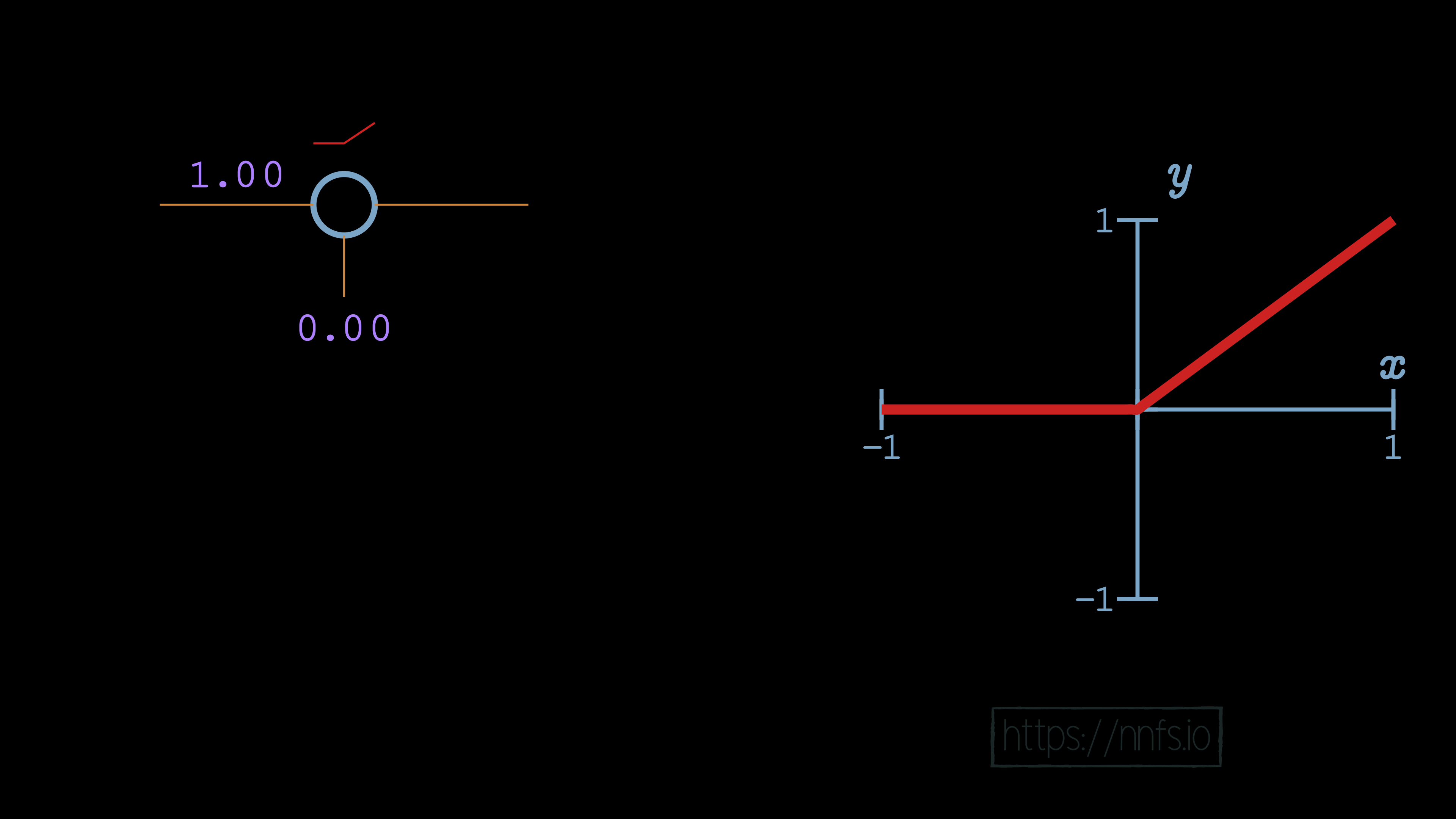
In this case, it looks just like the basic rectified linear function, no surprises yet! Now let’s set the bias to 0.50:

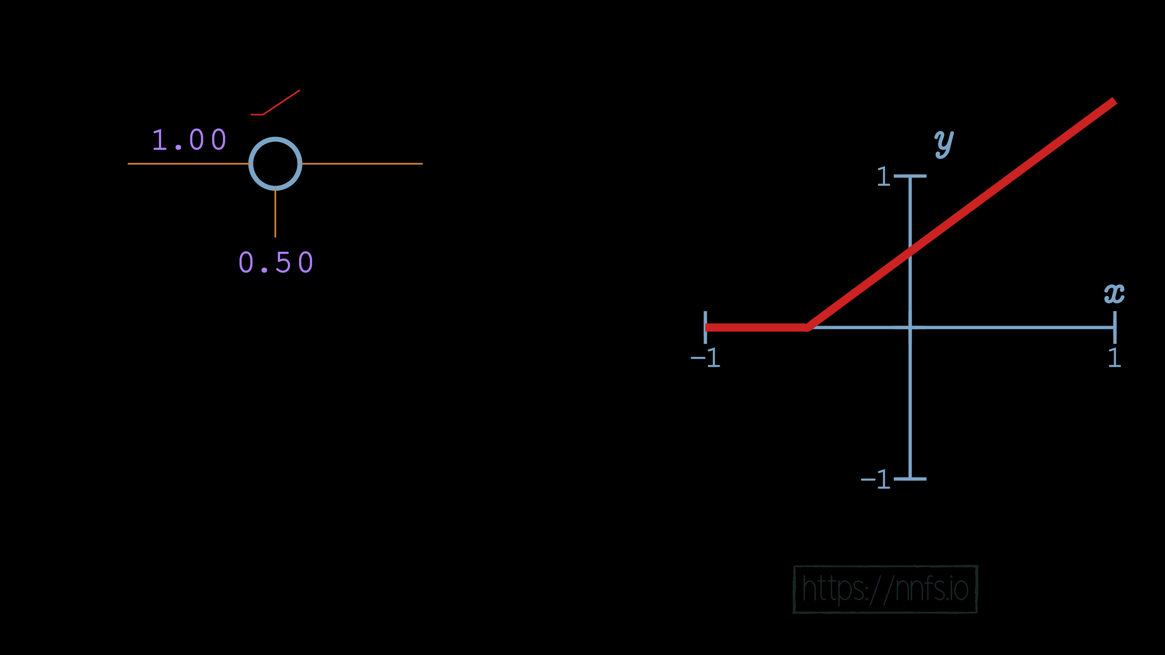
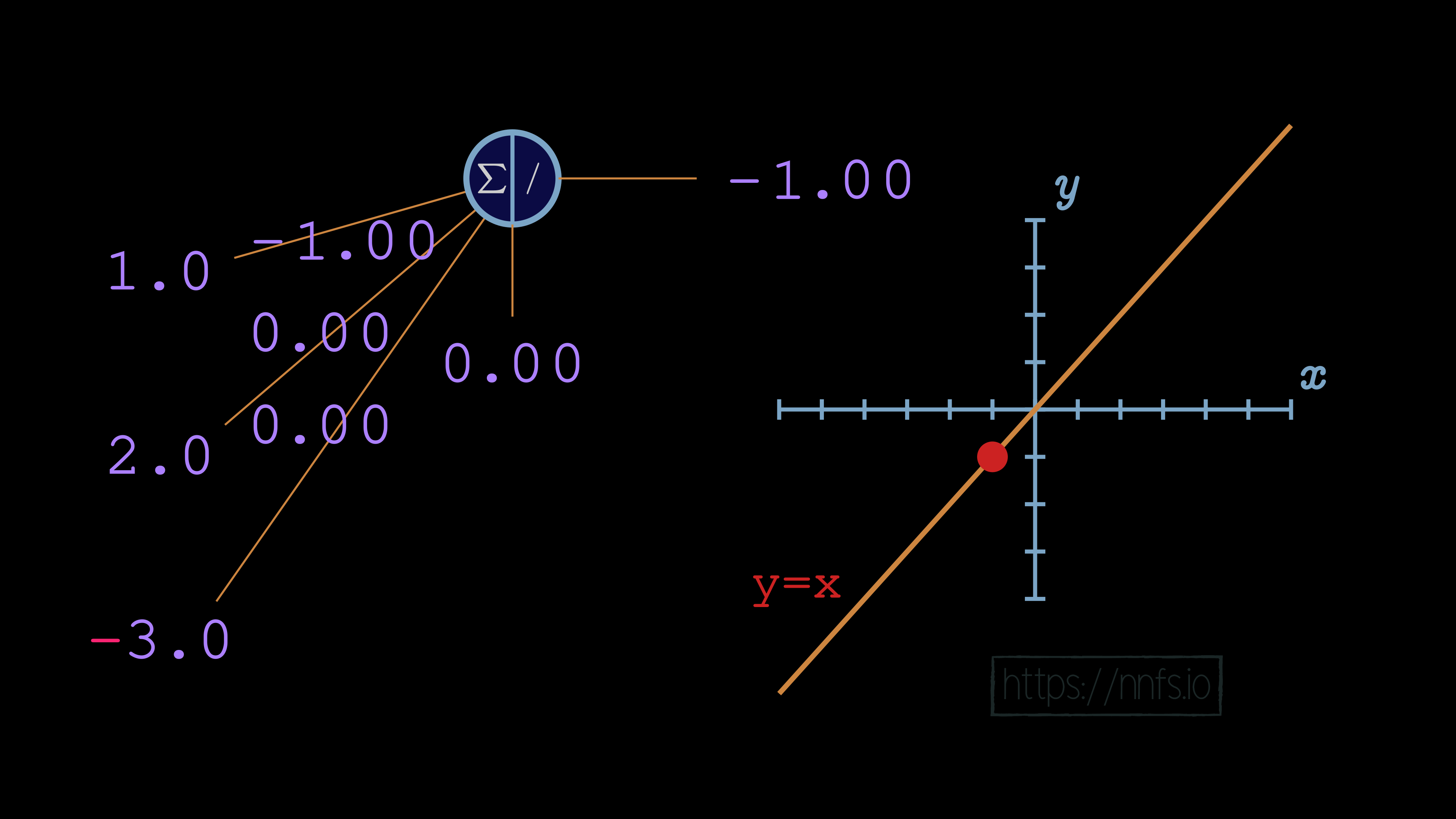
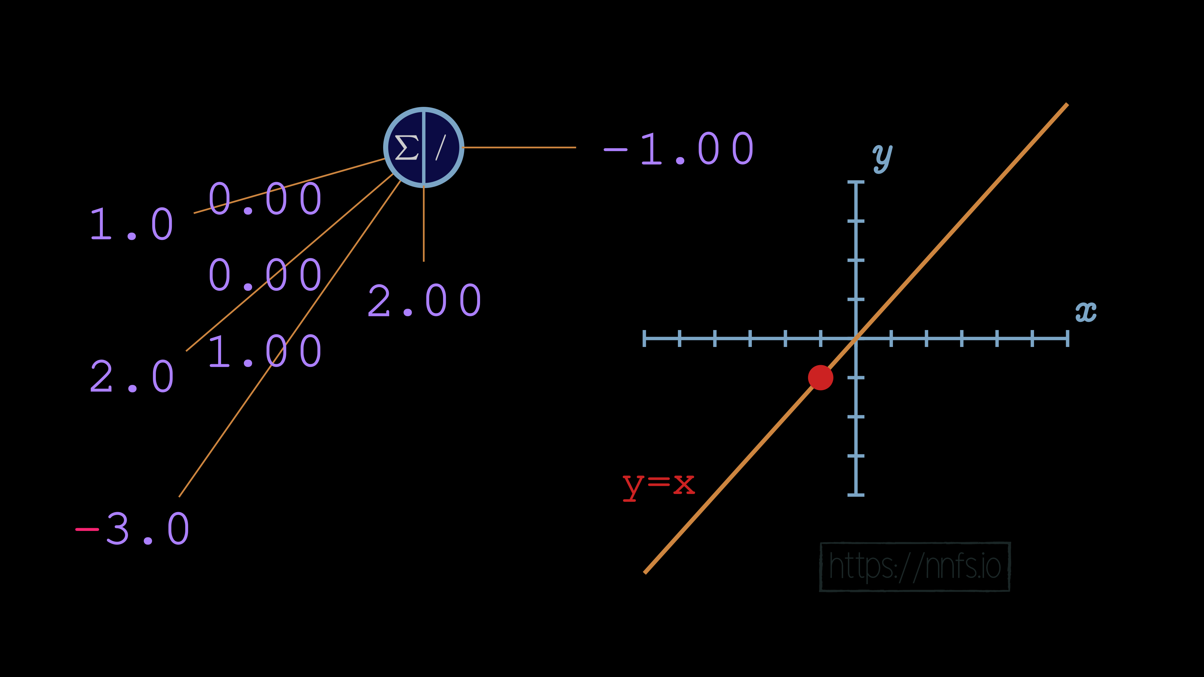
We can see that, in this case, with a single neuron, the bias offsets the overall function’s activation point horizontally. By increasing bias, we’re making this neuron activate earlier. What happens when we negate the weight to -1.0?

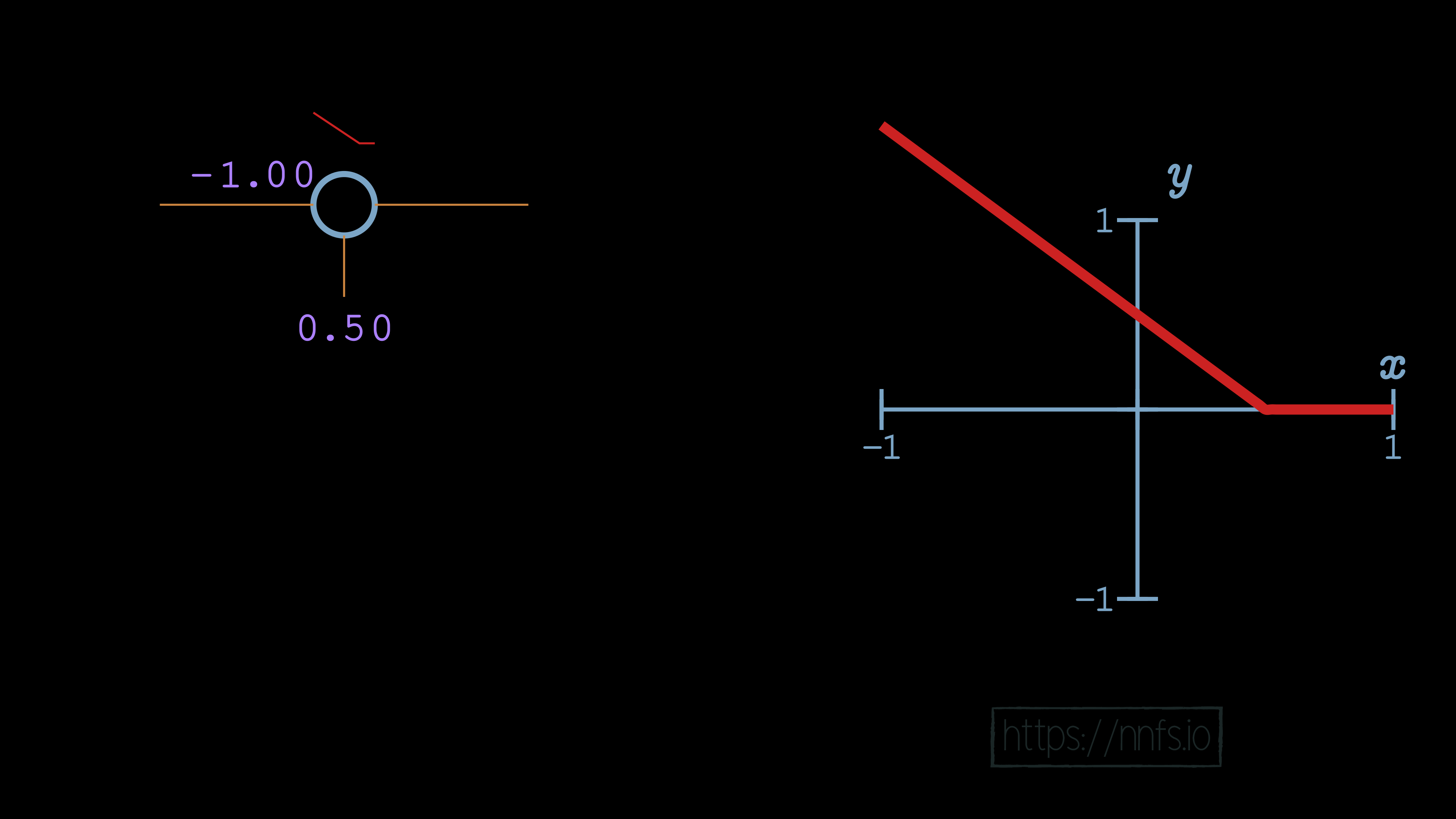
With a negative weight and this single neuron, the function has become a question of when this neuron deactivates. Up to this point, you’ve seen how we can use the bias to offset the function horizontally and how we can use the weight to influence the slope of the activation, to the point of also being able to control whether the function is one for determining where the neuron activates, or where the neuron deactivates.

What happens when we have, rather than just the one neuron, a pair of neurons? For example, let’s pretend that we have 2 hidden layers of 1 neuron each. Thinking back to the y=x activation function, we unsurprisingly discovered that, no matter what chain of neurons we made, a linear activation function produced linear results. Let’s see what happens with our rectified linear activation function. We’ll begin with a weight of 1, and a bias of 0 for the 2nd neuron:

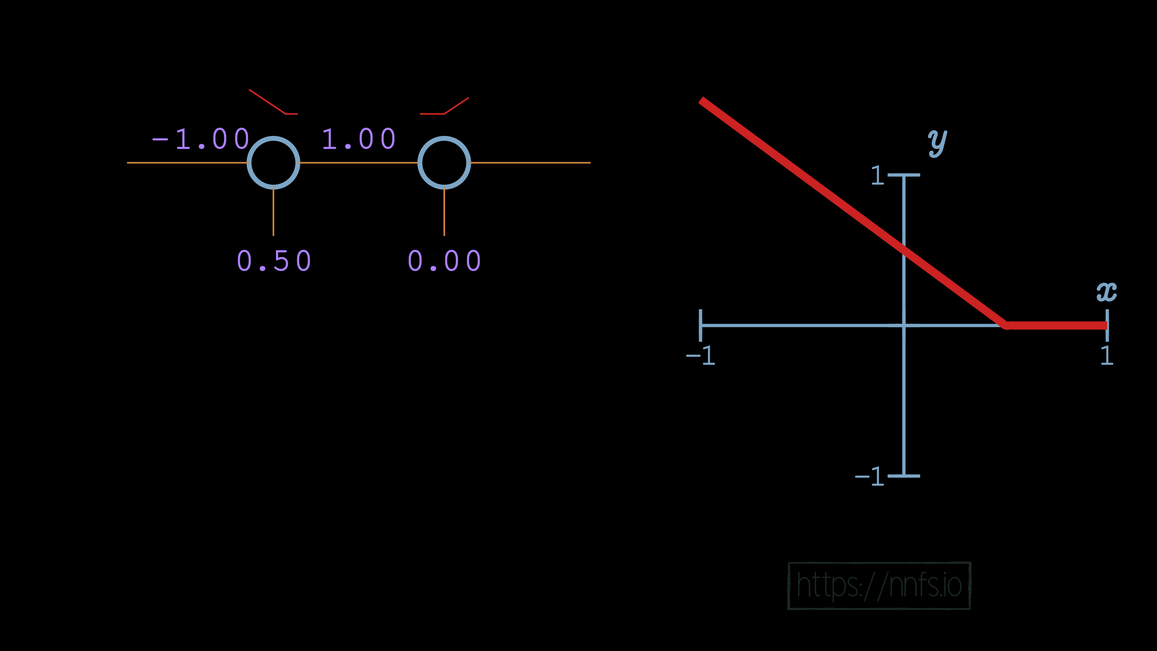
As we can see so far, there’s no change. This is because the 2nd neuron’s bias is doing no offsetting, and the 2nd neuron’s weight is just multiplying output by 1, so there’s no change. Let’s try to adjust the 2nd neuron’s bias now:

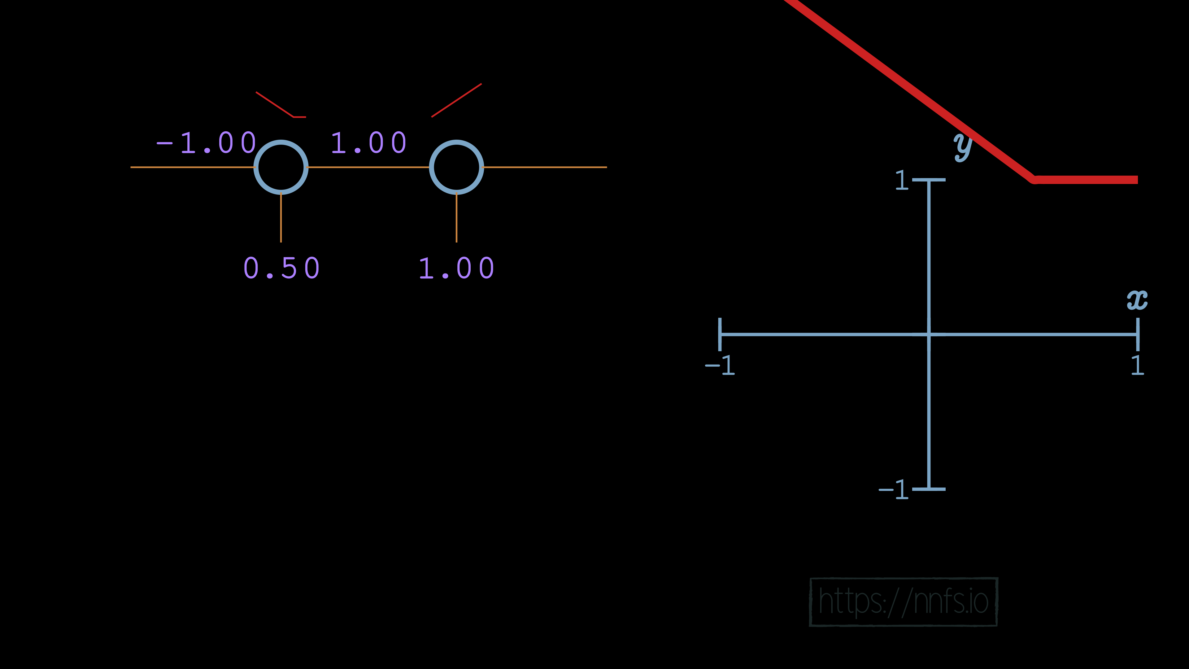
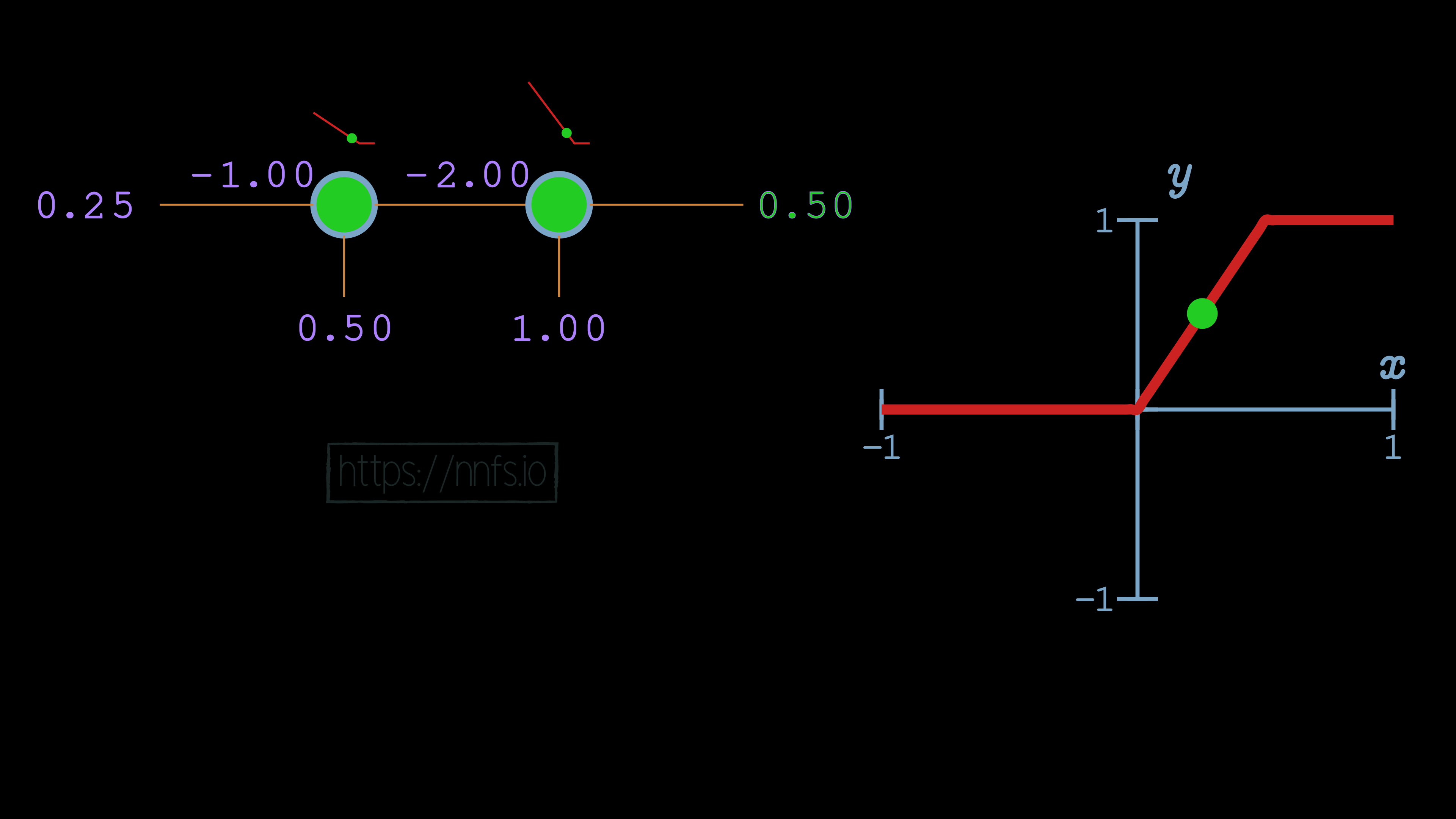
Now we see some fairly interesting behavior. The bias of the second neuron indeed shifted the overall function^{[e][f][g][h][i][j][k][l][m]}, but, rather than shifting it horizontally, it shifted the function vertically. What then might happen if we make that 2nd neuron’s weight -2 rather than 1?

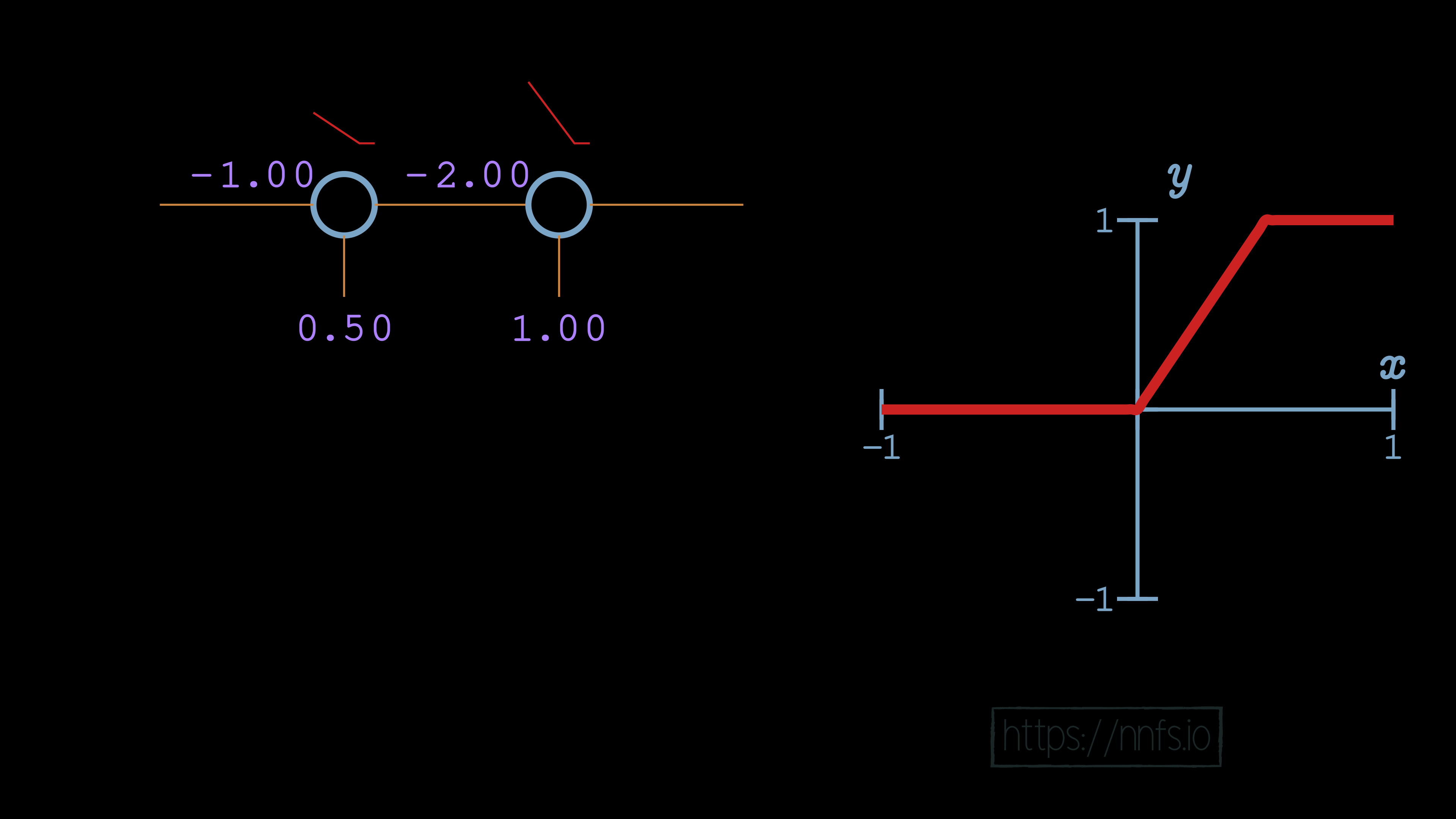
Something exciting has occurred! What we have here is a neuron that has both an activation and a deactivation point. When both neurons are activated, that is when their “area of effect” comes into play, and they produce values in the range of the granular, variable, output:

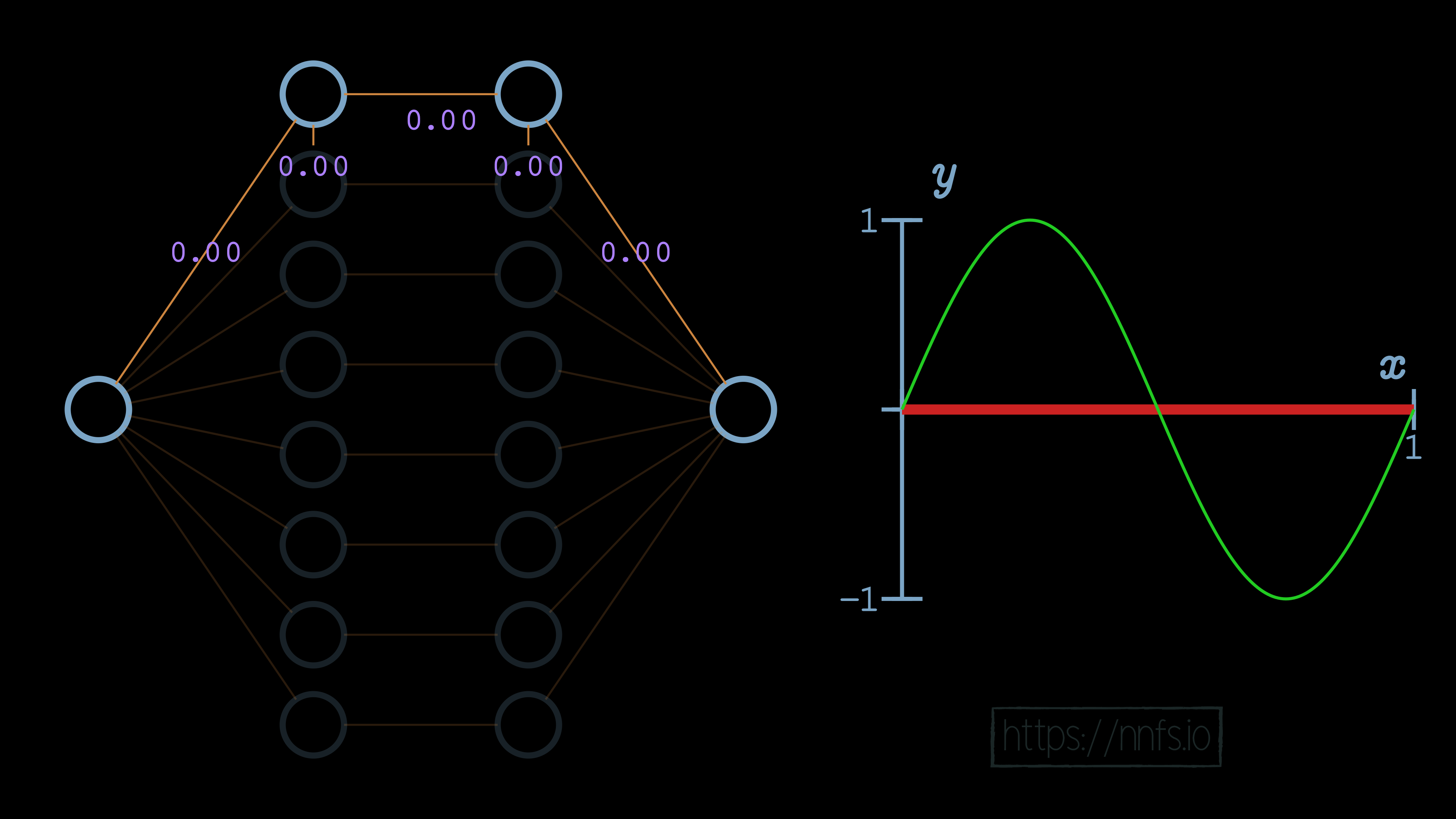
If any neuron in the pair is inactive, the pair will produce non-variable output. Let’s now take this concept, and use it to fit to the sine wave function using 2 hidden layers of 8 neurons each, and we can hand-tune the values to fit the curve. We’ll do this by working with 1 pair of neurons at a time, which means 1 neuron from each layer individually.

We will also set all weights to 0, except those directly connecting neurons at the same index for each hidden layer. To start, we’ll consider the first pair of neurons:

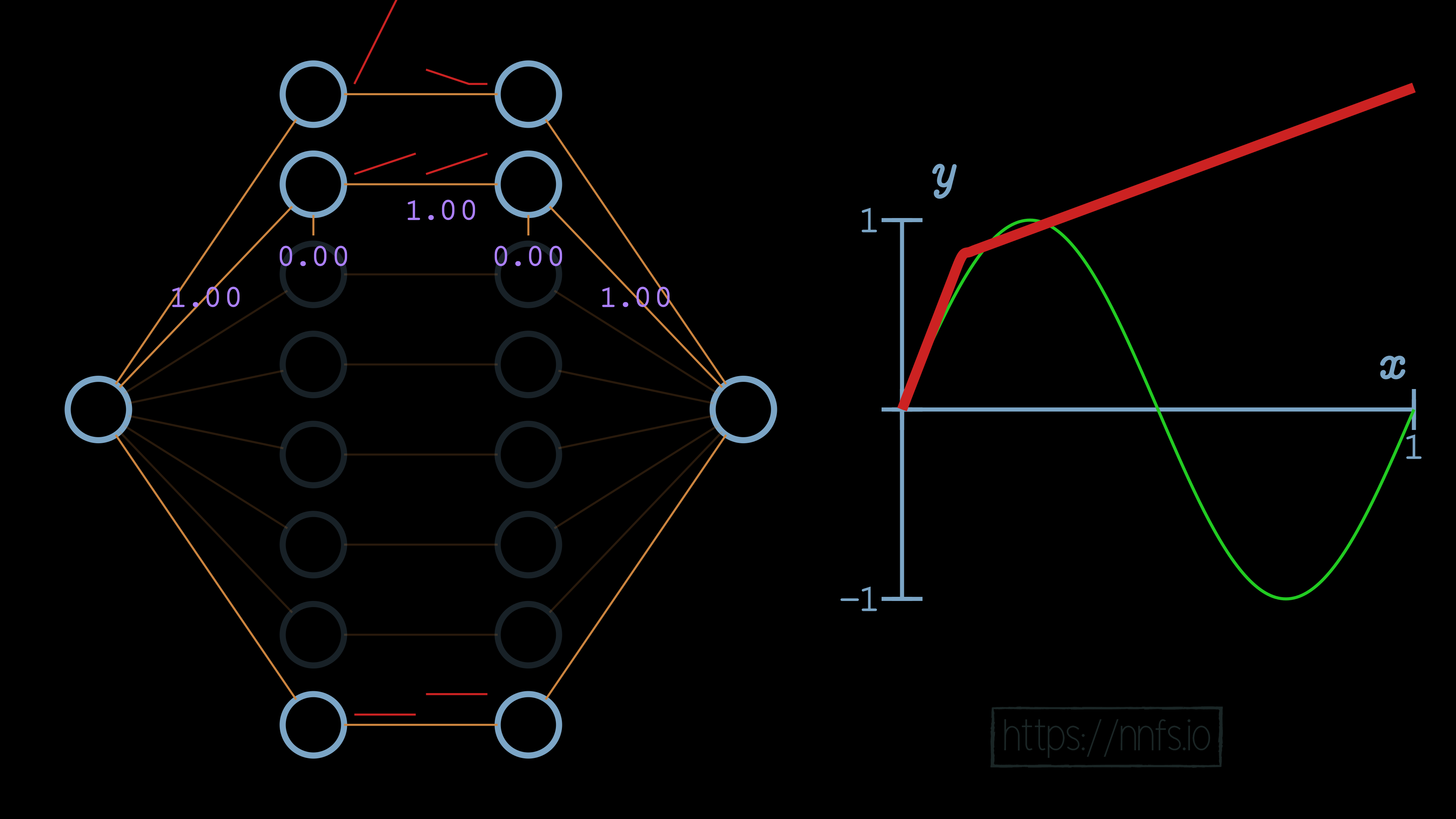
Next, we can set the weight for the hidden layer neurons and the output neuron to 1, and we can see how this impacts the output:

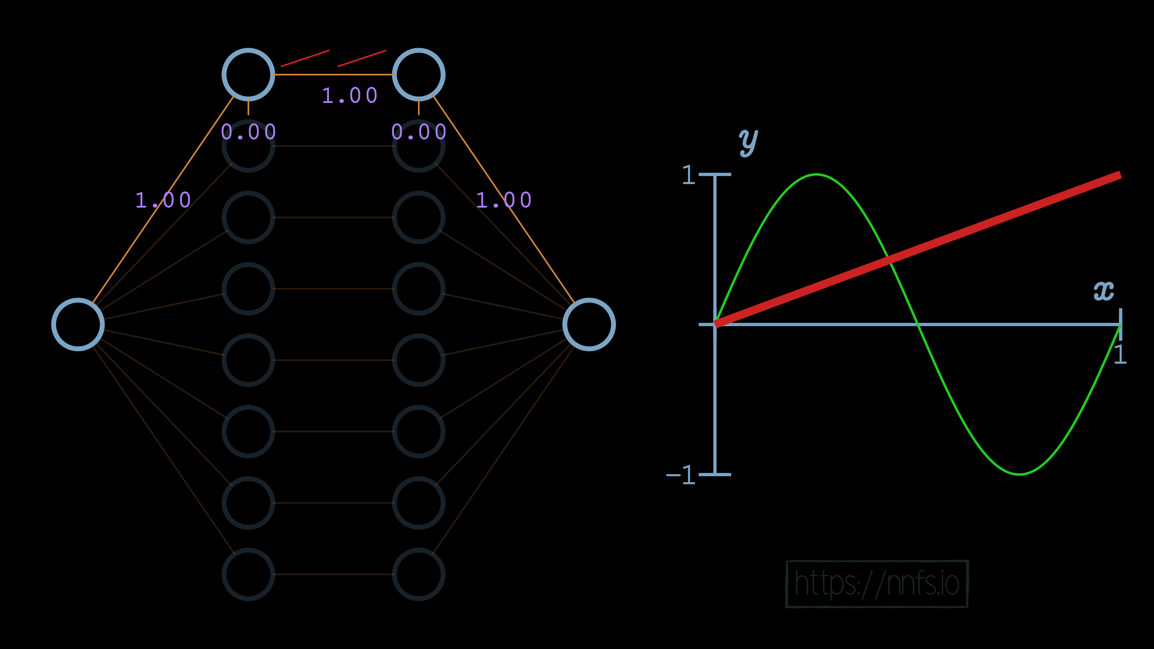
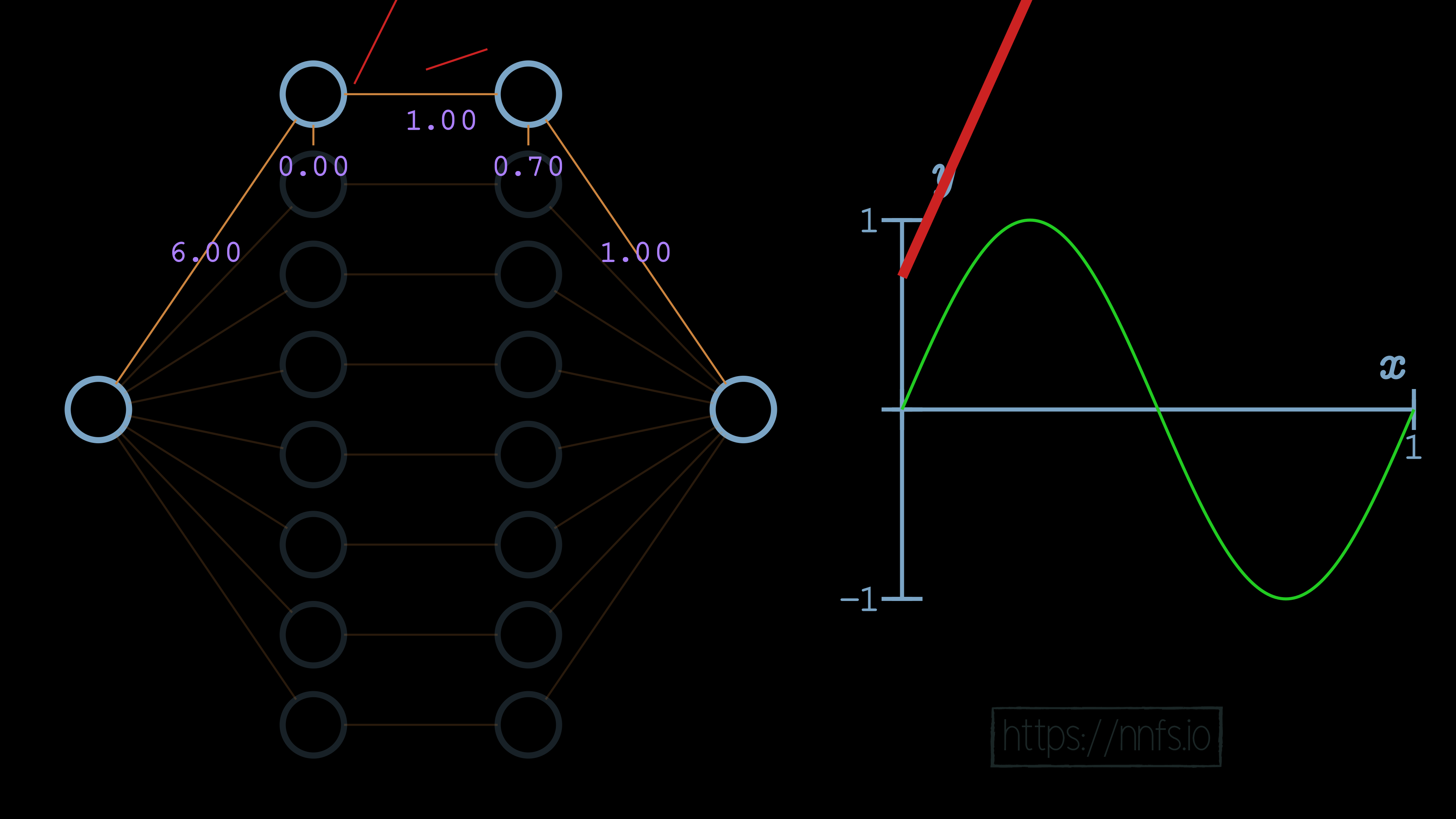
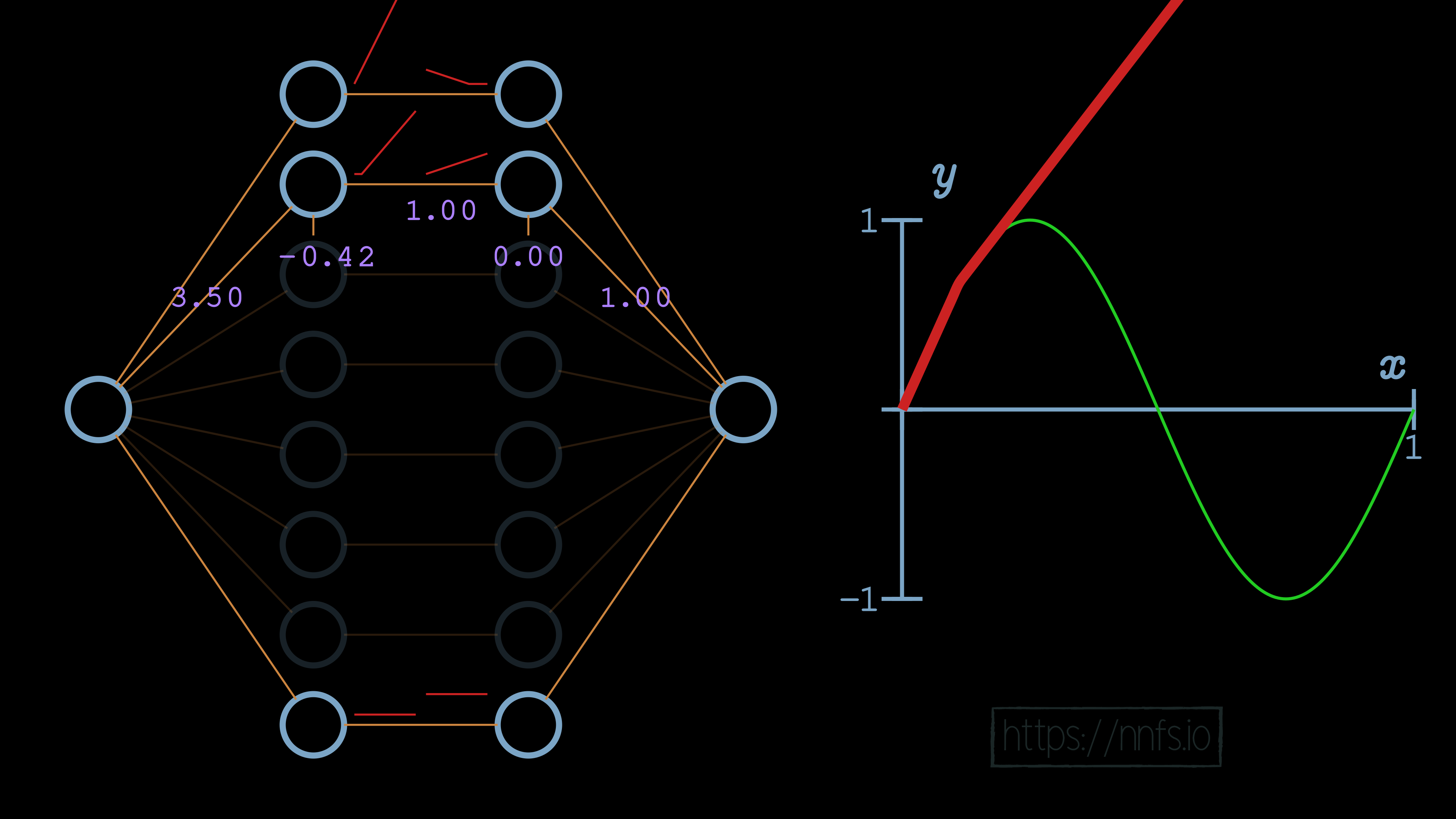
In this case, we can see that the slope of the overall function is impacted. We can further increase this slope by adjusting the weight for the first neuron of our hidden layers to 6.0:

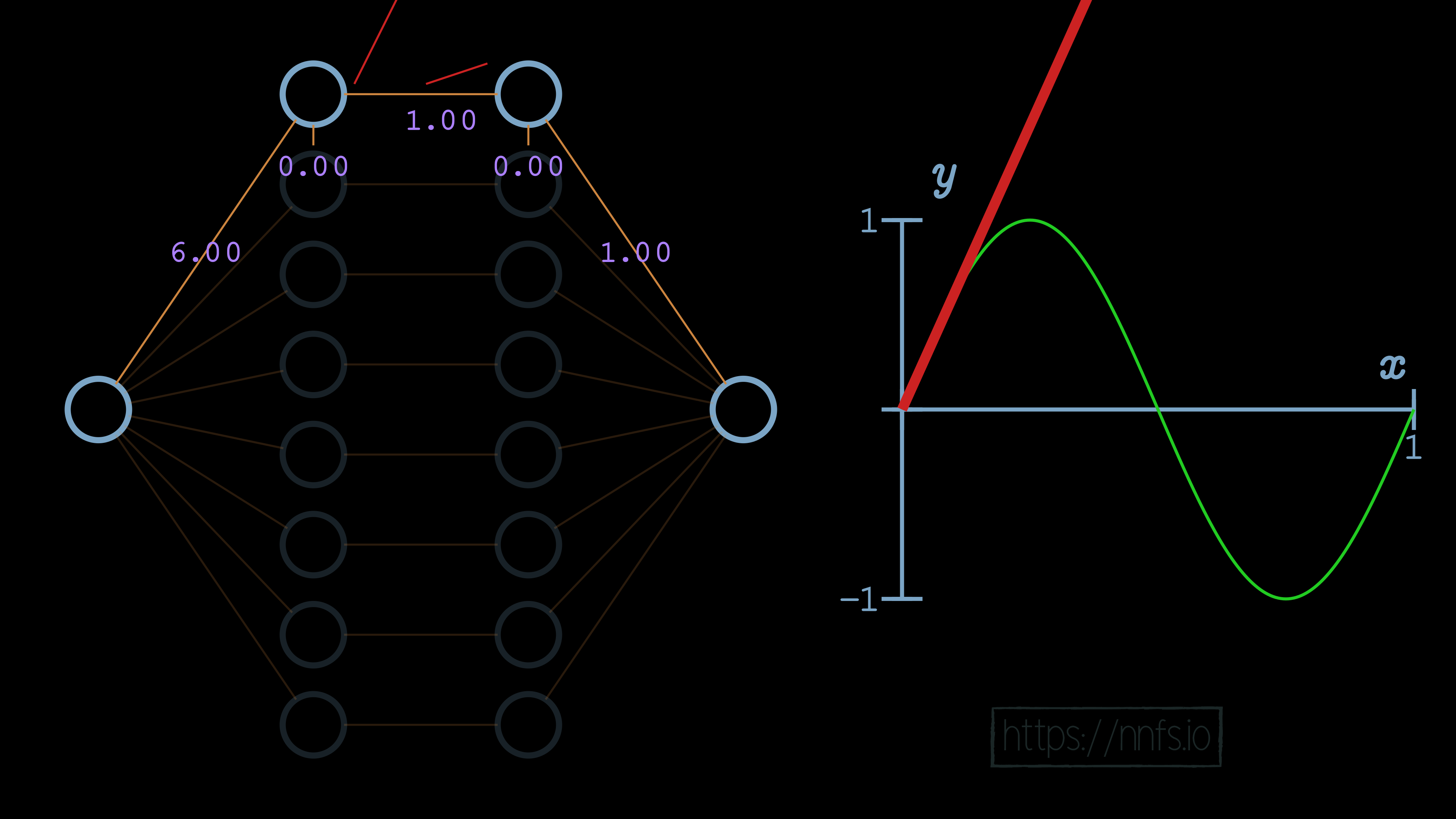
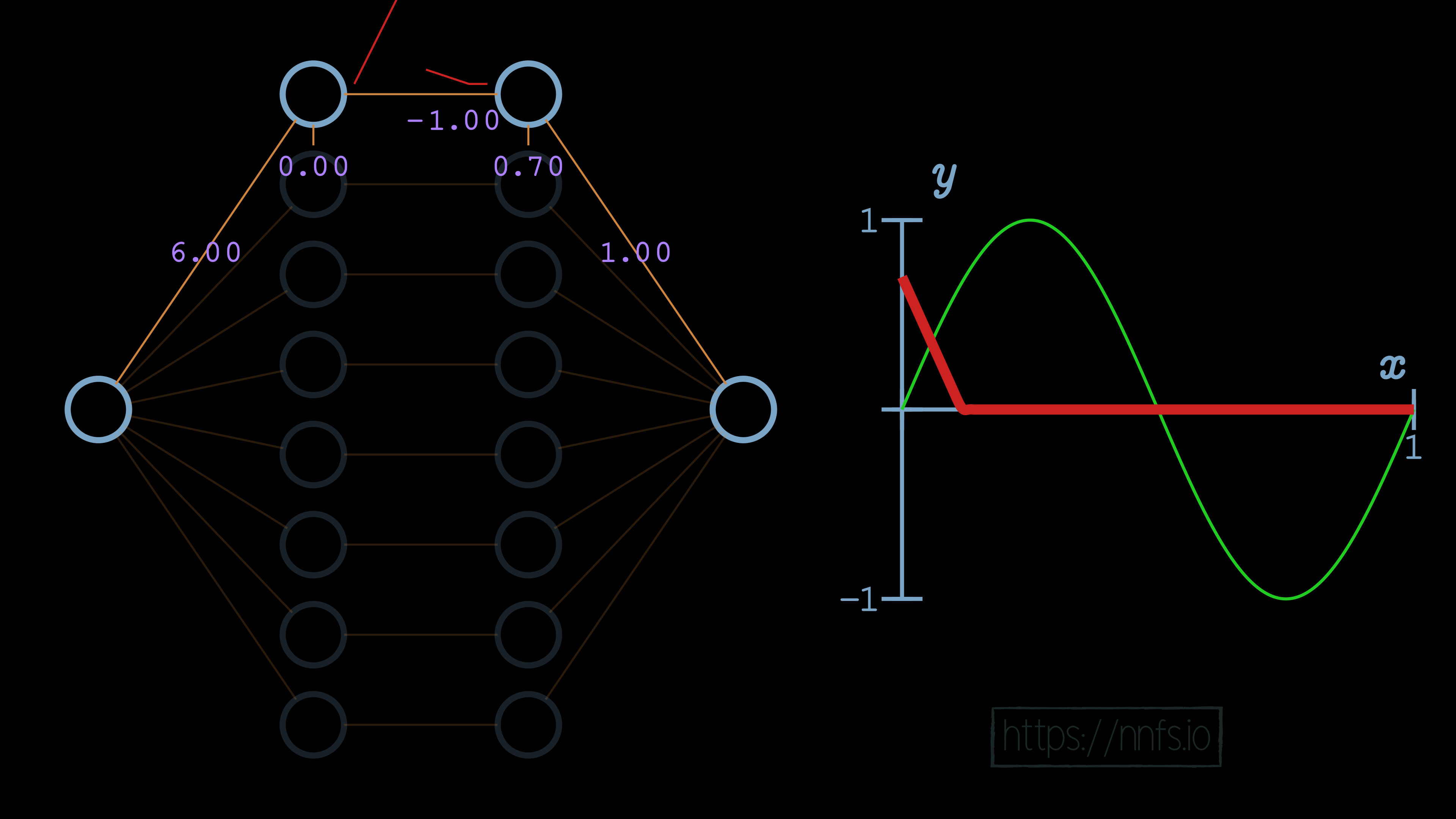
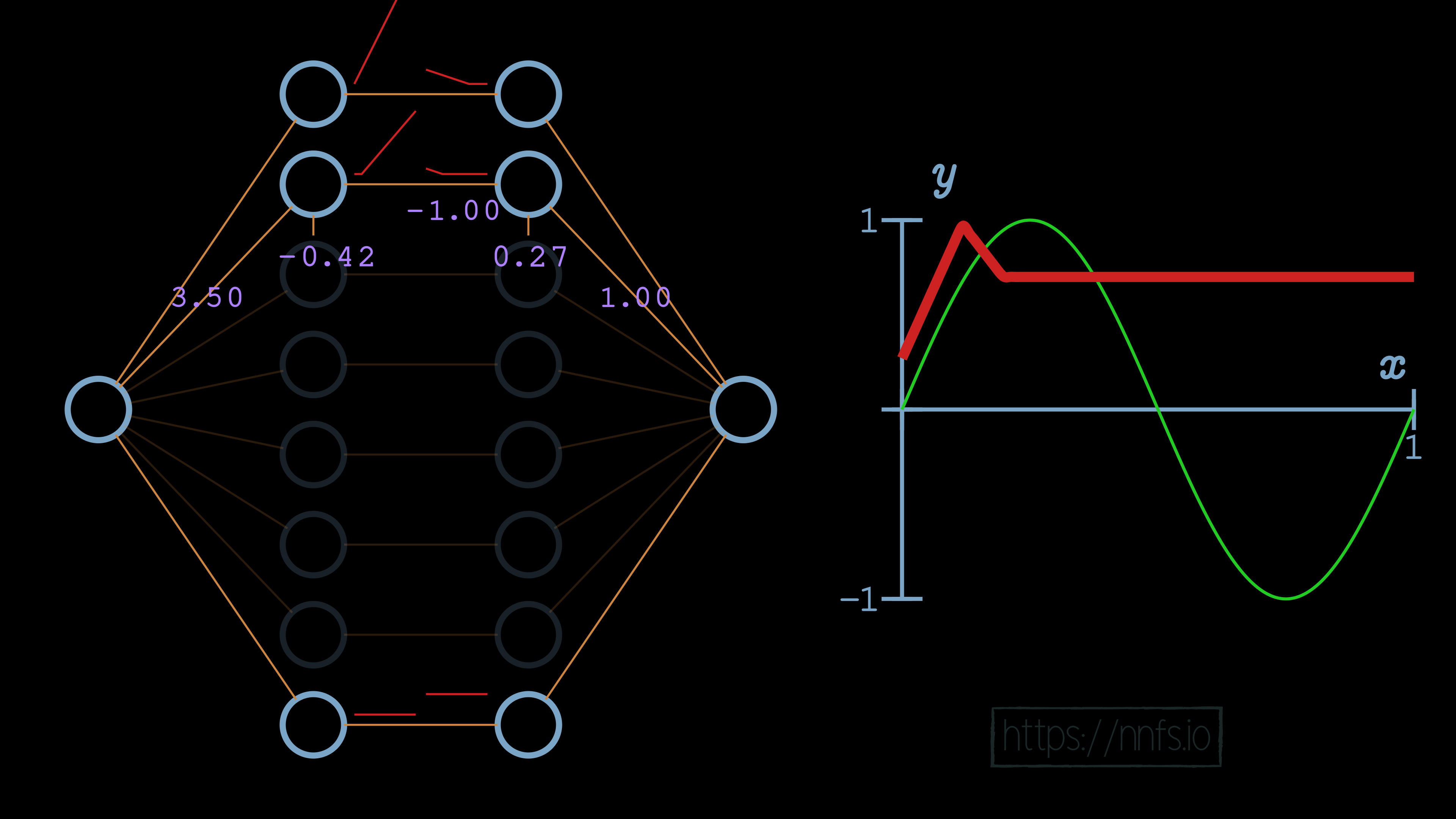
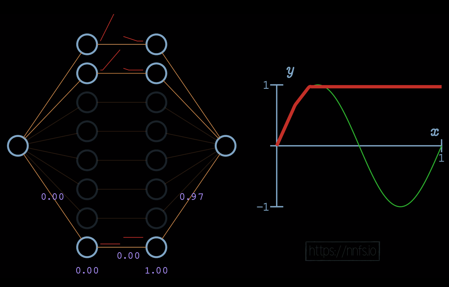
We can now see, for example, that the initial slope of this function is what we’d like, but we have a problem. Currently, this function never ends, because this neuron pair never deactivates. We can visually see already where we’d like the deactivation to occur. It’s where the red fitment line (our current neural network) diverges initially from the green sine wave. So now, while we have the correct slope, we need to set this spot as our deactivation point. To do that, we start by increasing the bias for the 2nd neuron of the hidden layer pair to 0.70. Recall that this offsets the overall function vertically:

Now we can set the weight for the 2nd neuron to -1, causing a deactivation point to occur, at least horizontally, where we want it:

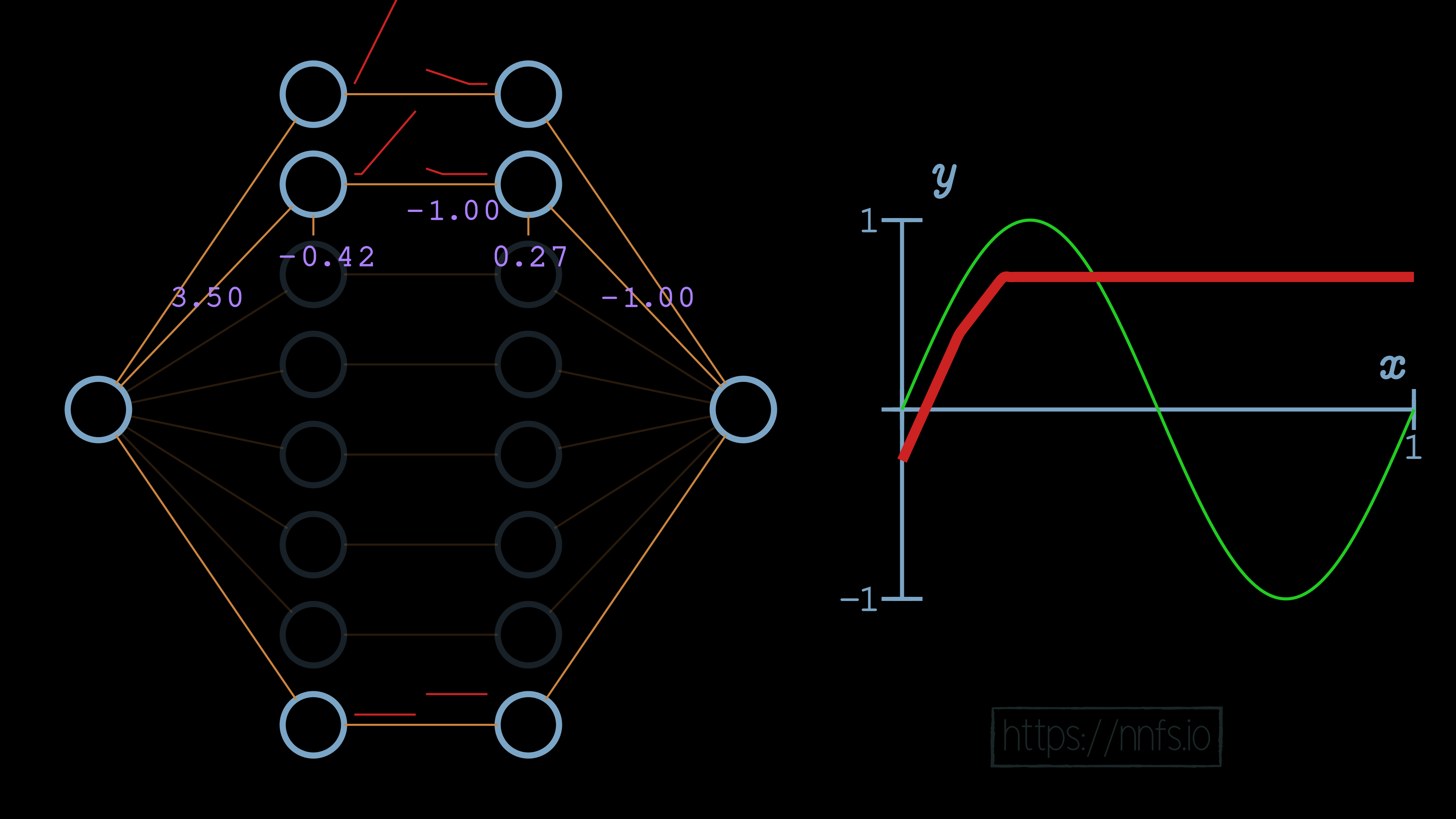
Now we’d like to flip this slope back. How might we flip the output of these two neurons? It seems like we can take the weight from these neurons, which is currently a 1.0, and just flip it to a -1, and that would flip the function:

^{[p][q][r][s][t][u][v][w][x][y]}

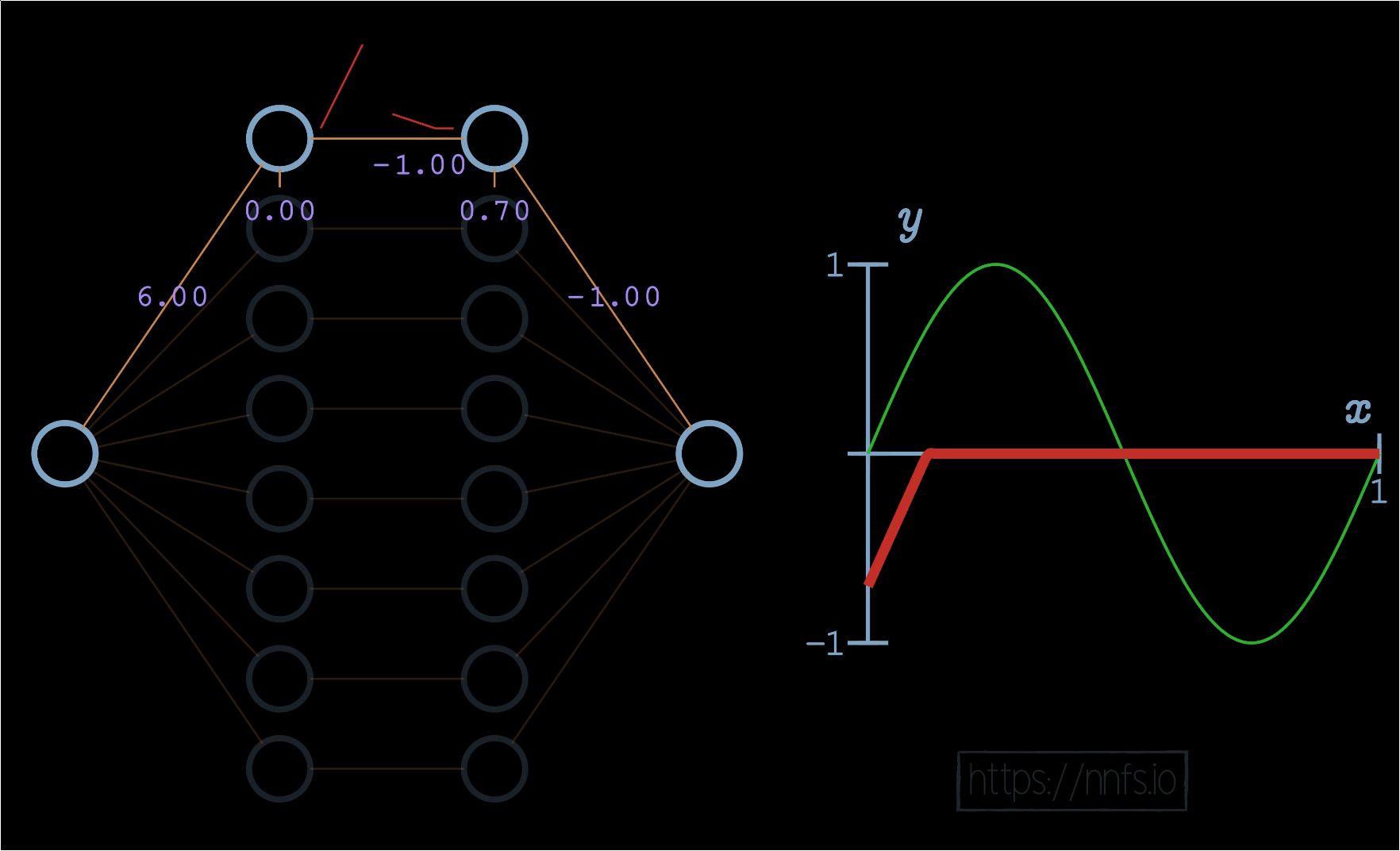
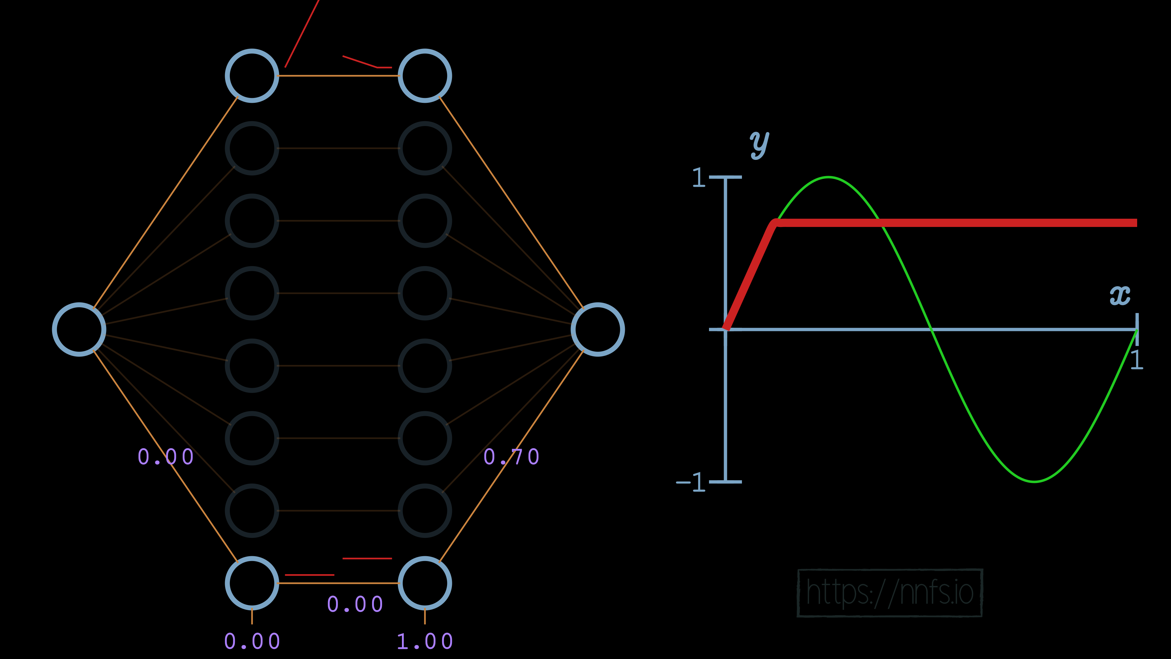
We’re certainly getting closer to making this first section fit how we want. Now, all we need to do is offset this up a bit. For this hand-optimized example, we’re going to use the first 7 pairs of neurons in the hidden layers to create the shape of the sine wave, then the bottom pair to offset everything vertically. If we set the bias of the 2nd neuron in the bottom pair to 1.0 and the weight to the output neuron as 0.7, we can vertically shift the line like so:

At this point, we have completed the first section with an “area of effect” being the first upward section of the sine wave. We can start on the next section that we wish to do. We can start by setting all weights for this 2nd pair of neurons to 1, including the output neuron:

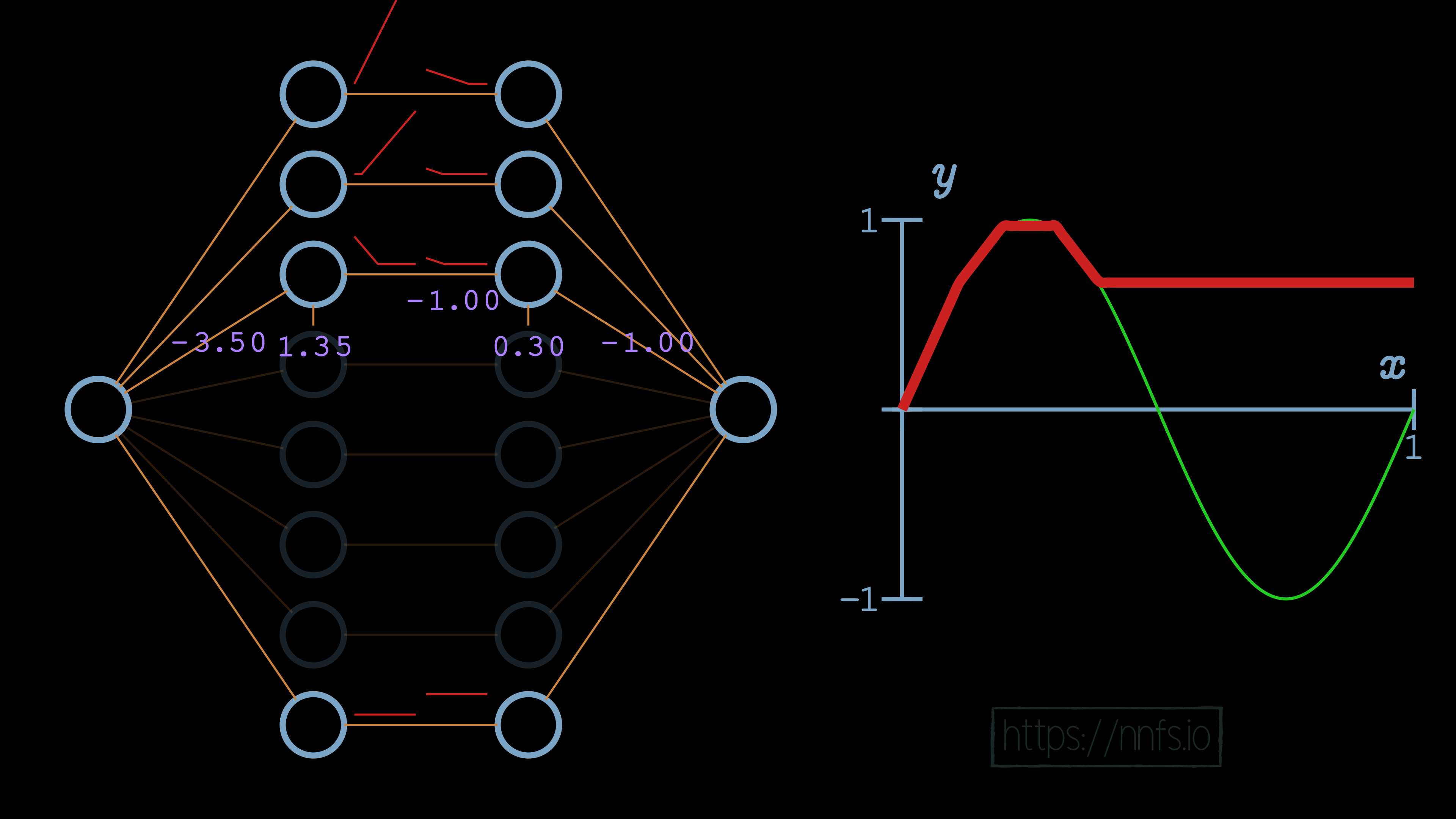
At this point, this 2nd pair of neurons’ activation is beginning too soon, which is impacting the top pair that we already aligned. To fix this, we want to adjust the function horizontally. As you can recall from earlier, we adjust the first neuron’s bias in this neuron pair to achieve this. Also, to modify the slope, we’ll set the weight coming into that first neuron for the 2nd pair, setting it to 3.5, which is the same method we used to set the slope for the first section, which is controlled by the top pair of neurons in the hidden layer. Currently:

^[z][aa]

We will use the same methodology as we did with the first pair now, to set the deactivation point. We’ll set the weight for the 2nd neuron in the hidden layer pair to -1 and the bias to 0.27.

Then we can flip this section’s function, again the same way we did the first, by setting the weight to the output neuron from 1.0 to -1.0:

And again, just like the first pair, we will use the bottom pair to fix the vertical offset:

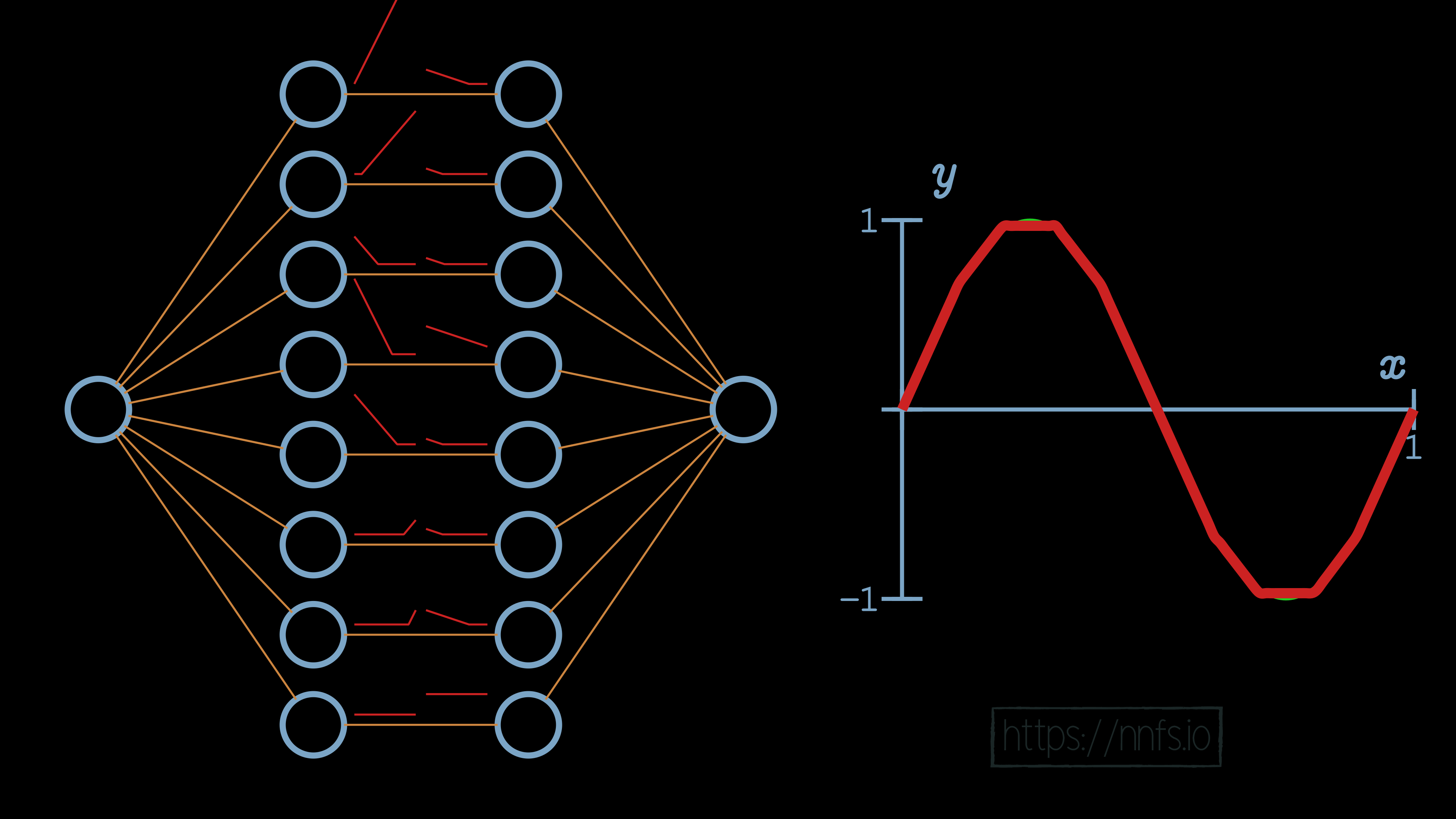
We then just continue with this methodology. For the top section, we’ll just leave it flat, which means we will only begin the activation for the 3rd pair of hidden layer neurons when we wish for the slope to start going down:

This process is simply repeated for each section, giving us a final result:

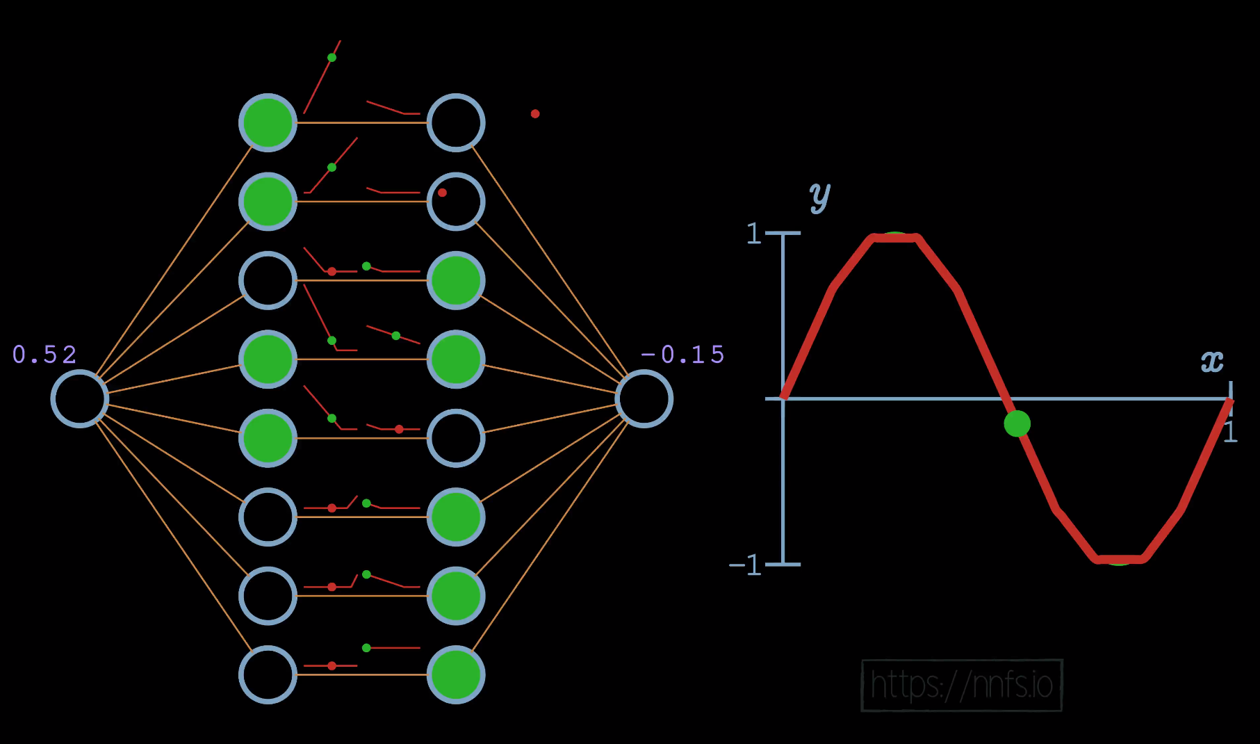
We can then begin to pass data through to see how these neuron’s areas of effect come into play only when both neurons are activated based on input:

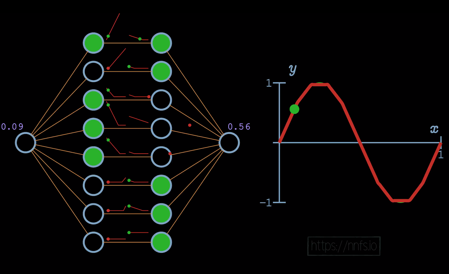
In this case, given an input of 0.08, we can see the only pairs activated are the top ones, as this is their area of effect. Continuing with another example:

As you can see, even without any of the other weights, we’ve used some crude properties of a pair of neurons with rectified linear activation functions to fit this sine wave pretty well. If we enable all of the weights now and allow a real optimizer to train, we can see even better fitment: